Overview
In this project, we built a simple rasterizer based on triangles. The final program is a functional vector graphics renderer that can take in a simplfied version of SVG (Scalable Vector Graphics) files and apply PNG textures to them. Within this program, we first drew triangles with a rasterization technique but since this implementation is simple, this resulted in aliasing artifacts and jaggies in the images. To solve this, we incorporated supersampling which allowed multiple sample points to be taken within each pixel instead of just sampling one point per pixel. There is less aliasing present within the images rasterized but we wanted to have the ability to orient them differently, so we implemented transformation functionality (rotation). Afterwards, we utilized the barycentric coordinate system to help us determine colors inside a triangle since previously, we were only working with a single color within the triangle. This system also allowed us to sample points from texture space, enabling us to apply textures onto a surface after transforming between the image and texture coordinates. We are able to differentiate which sampling method to utilize (nearest vs bilinear) within texture mapping with antialiasing. Specifically, the close and further distances in an image creates jaggies and aliasing which we solved by using level sampling (mipmap) — the ability to sample from textures with different precision levels.
I've never worked with graphics before so I thought it was fascinating how we were able to completely work our way down the rasterization pipeline, starting from drawing triangles to coloring them, rotating, then applying textures. The codebase was a bit difficult initially to work through since I wasn't familiar with the different methods provided but after spending hours on this project, it was very rewarding to see the output of my results through the cool images rasterized, antialiased, and texturized!
Task 1: Drawing Single-Color Triangles
Implementation
To rasterize triangles, we first need to determine the boundary box to account for edges and find the boundary of where a point would be included and where it won't. The bounding box is defined as the rectangle from \((x_{\text{min}}, y_{\text{min}})\) to \((x_{\text{max}}, y_{\text{max}})\). \(x_{\text{min}}\) is determined as the minimum x coordinate of the vertices passed in as input by using the min and floor functions. \(x_{\text{max}}\) is similarly calculated but with the max function instead. The same process was done for the y coordinate. These values represent the smallest and largest x and y values out of the points given as input. Therefore, our algorithm only looks at points/pixels within the bounding box of the triangle.
Next, we implemented the line test method taught in the lecture to determine whether a point laid inside or outside of the triangle. To do this, we initially created a lambda function that determined whether the point is to the left, right, or on the edge/line \(AB\). If the point is on the same side of each triangle edge, this meant that the point is inside the triangle. Later on the project, we created a separate helper function defined as point_inside() that did the line test calculation for each line of the triangle outside of rasterize_triangle() for more convenient usage. Our implementation ensures that the line test would work regardless of the winding order of the vertices.
After that, we now know the boundary box so we're able to iterate over every single pixel using a double for loop. Using our helper function, if the point is in the triangle, we send the according color to the frame buffer using fill_pixel(). This color could be a given color or sampled from a texture.

Example of basic triangles with aliasing displayed
Task 2: Antialiasing by Supersampling
Implementation
In traditional rendering and in Task 1, we sampled the point in the middle of the pixel by adding 0.5 to the x and y axis to determine the pixel's color. This can lead to aliasing issues especially along edges and curves, creating jaggies which is displayed with our results from rasterization done in Task 1. With supersampling, multiple sample points are taken within each pixel instead of just sampling one point per pixel. We divide each pixel into 4, 9, and 16 squares — essentially 4, 9, and 16 points inside each pixel. Since each pixel is divided into subsamples, each is essentially treated as their own points/"pixels" and were thus subject to the same sampling method of whether the point was inside or outside the triangle.
However, we aren't able to directly apply this to the screen because we have fewer screen pixels than our data structure. We averaged the color of the sampled points to create a new color for each pixel. The color was based on the "area" of the single sample that was covered by the triangle. To store the supersamples, we used the existing data structure/variable sample_buffer which is essentially a std::vector that is the internal color sample buffer containing all samples. Notably, the number of elements in the buffer = width * height * sample_rate.
Supersampling is useful because creates better detail in our triangles by "smoothening out" the edges by generating intermittent colors between high-frequency pixels. Instead of only 1 sample per pixel, the averaging process helps reduce aliasing artifacts and produces smoother transitions between colors, resulting in a better visual representation of the triangle.
For the rasterization pipeline, we made a few modifications to the rasterization pipeline in the process. Specifically, we utilized the sample_rate variable previously defined to specify the number of samples per pixel. In the resolve_to_framebuffer function, instead of directly copying colors from the sample buffer to the framebuffer, colors from all sample points within each pixel are averaged to produce the pixel's final color. We also updated set_sample_rate(), set_framebuffer_target() and resolve_to_framebuffer() to account for the changes in sample_rate. An important note is that despite supersampling enabling "smoother" and more detailed images, it increases computational cost since more samples need to be processed for each pixel.
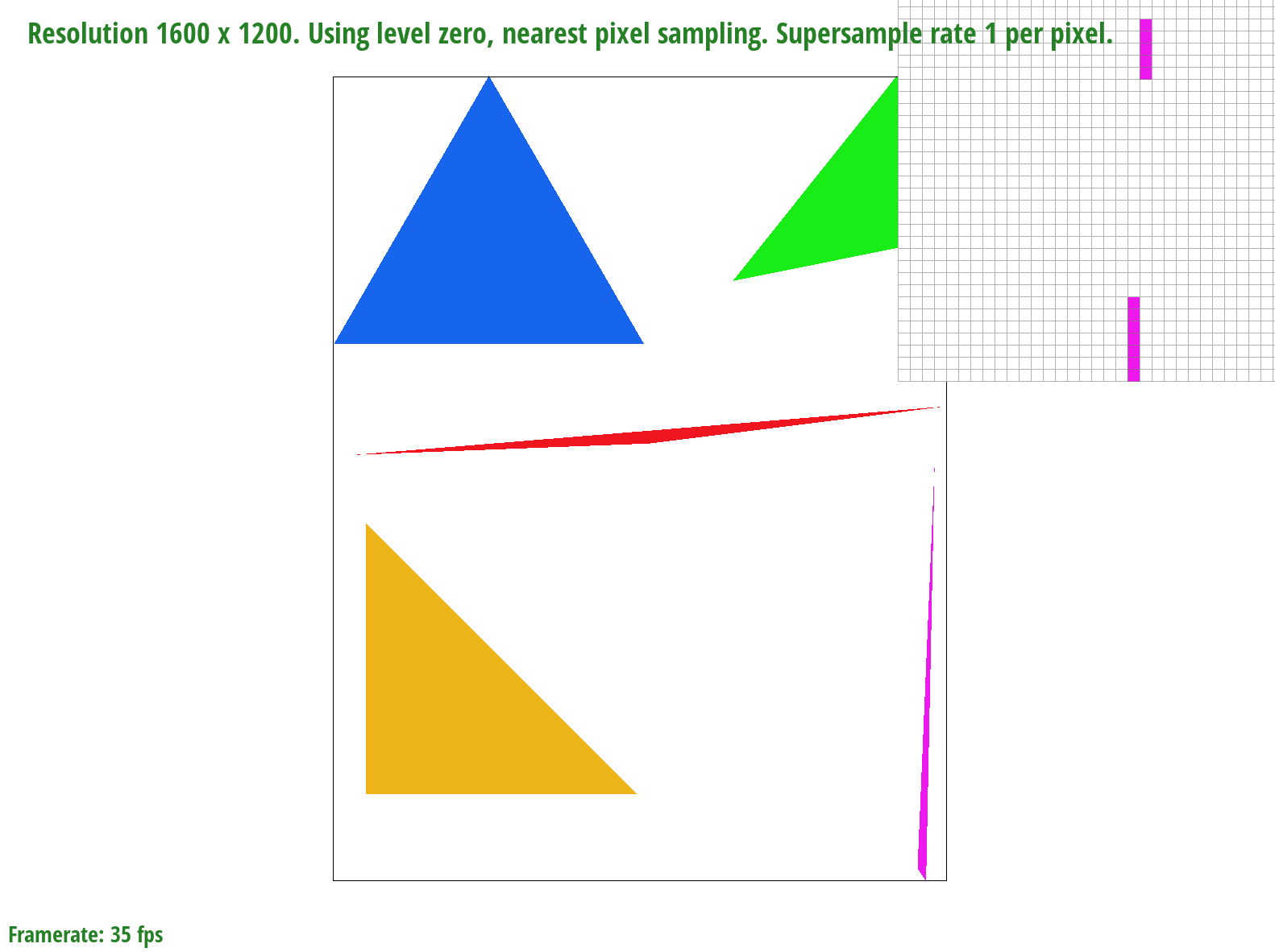
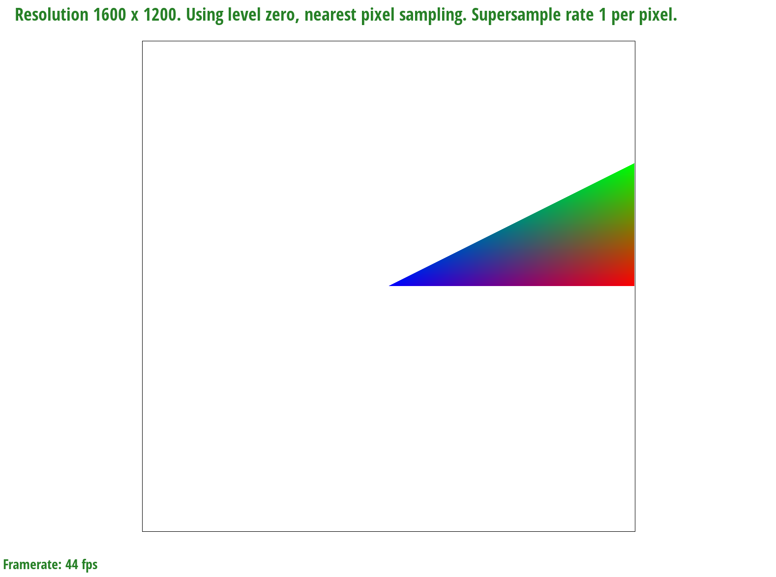
basic/test4.svg with the default viewing parameters and sample rate of 1 per pixel
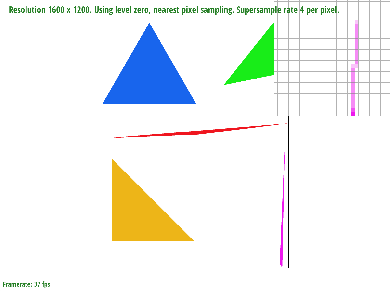
basic/test4.svg with the default viewing parameters and sample rate of 4 per pixel
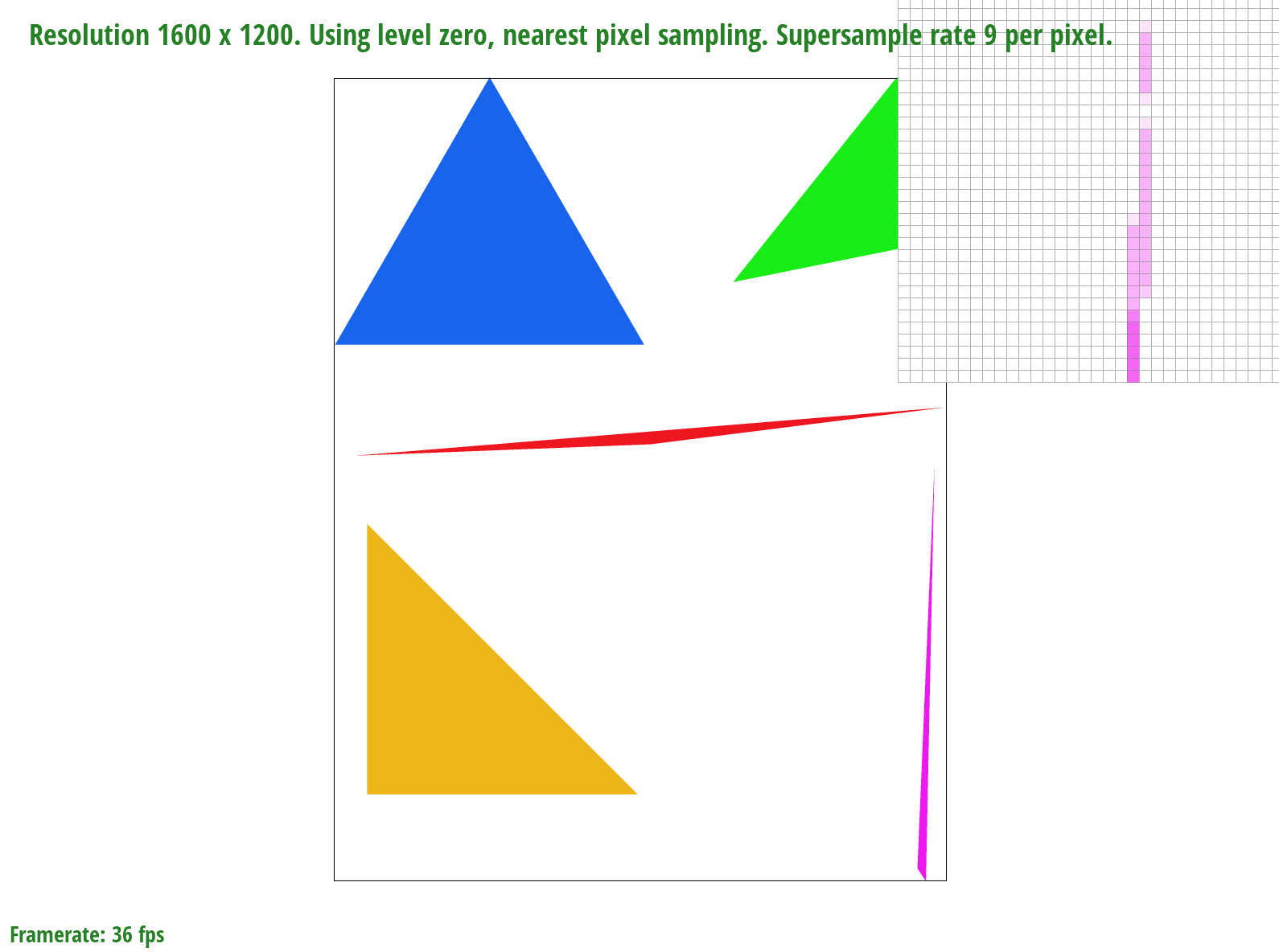
basic/test4.svg with the default viewing parameters and sample rate of 9 per pixel

basic/test4.svg with the default viewing parameters and sample rate of 16 per pixel
We zoom in on a very skinny corner of the pink triangle. When we only sample once per pixel, entire pieces of the triangle are missing but as we sample more times per pixel, more of the triangle "appears"/"fills in". This is because of the averaging color effect that reduces aliasing - for example, if a sample was 50% covered by the triangle, it would be closer to 50% the saturation of the triangle color.
Task 3: Transforms
Implementation
For this version of the cubeman, we wanted to make it wave. To do this, we moved one arm down closer to its side, and made the other arm bend so that it appears like the cubeman is waving. We also changed the colors of the objects that make up the cubeman to give off a more human-like appearance with clothes.
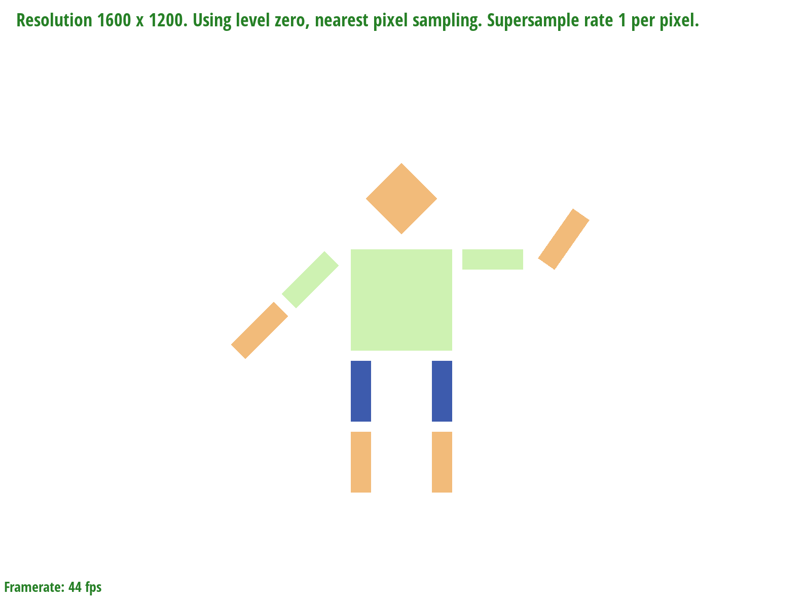
Screenshot of our robot
Task 4: Barycentric Coordinates
Implementation
Barycentric coordinates help us to linearly interpolate coordinates so that a texture or color mapping is smooth and even without jagged lines. When we use barycentric coordinates, we are finding the exact distance of the point and what combination of values is needed to get what we want at that point. We can take this image of a colored triangle as an example.
Screenshot of blended colored triangle
We start off as each corner of the triangle being red, green, and blue. Then, barycentric coordinates helps us calculate the exact ratio of how much red, green, and blue we need at a specific point in the triangle, and colors it that color. This happens for the whole triangle until it is fully smoothly shaded.
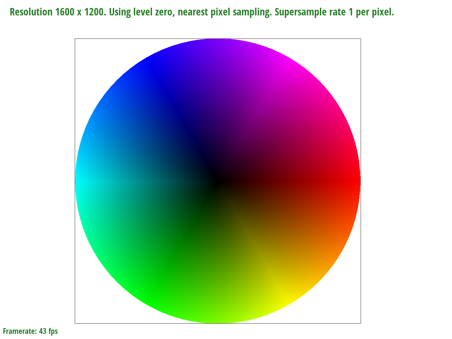
Screenshot of the colorwheel generated by the interpolated coordinates
One issue we came across with generating this image is that there seems to be a thin white line going through the circle when first rendered. However, if we move the circle slightly to the side, either the white line changes position, or it goes away altogether, which is shown in the image above. We first thought this was an issue with our bounding box since it could affect the edges, which may cause the line to occur. We tried flooring the values and also changing them from floats the doubles, but nothing was able to fix it. We think it could be an issue internally with the rendering and creation of the window, since there are positions where the full circle is colored in and interpolated correctly.
Task 5: "Pixel sampling" for Texture Mapping
Implementation
Pixel sampling is how translate from x-y coordinates for pixels to texel u-v coordinates. It's essentialy how we map textures onto triangles of the vector graphic - we're given the corresponding texture coordinates so we sample the color of a given point from a texture. When converting x-y to u-v, this results in a decimal value but we can only sample from integers. If we are using the nearest pixel sampling method, we sample from the nearest integer u and v coordinates. If we are using the bilinear method, we sample from the four closest u-v coordinates and use linear interpolation to create a weighted sample of neighbors in the horizontal and vertical directions for the new color.
The closer the point is to one of the corners, that corner's color will have a stronger influence on the fill color. Pixel sampling typically gives us better rendering since textures appear smoother as a result of averaging texels - less jumps between neighboring pixels.
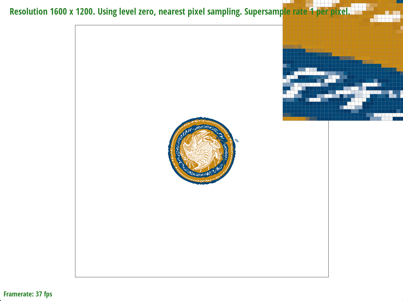
Nearest sampling at 1 sample per pixel
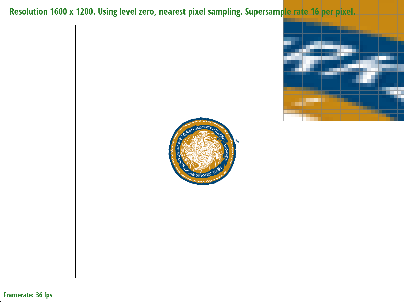
Nearest sampling at 16 samples per pixel
Bilinear sampling at 1 sample per pixel
Bilinear sampling at 16 samples per pixel
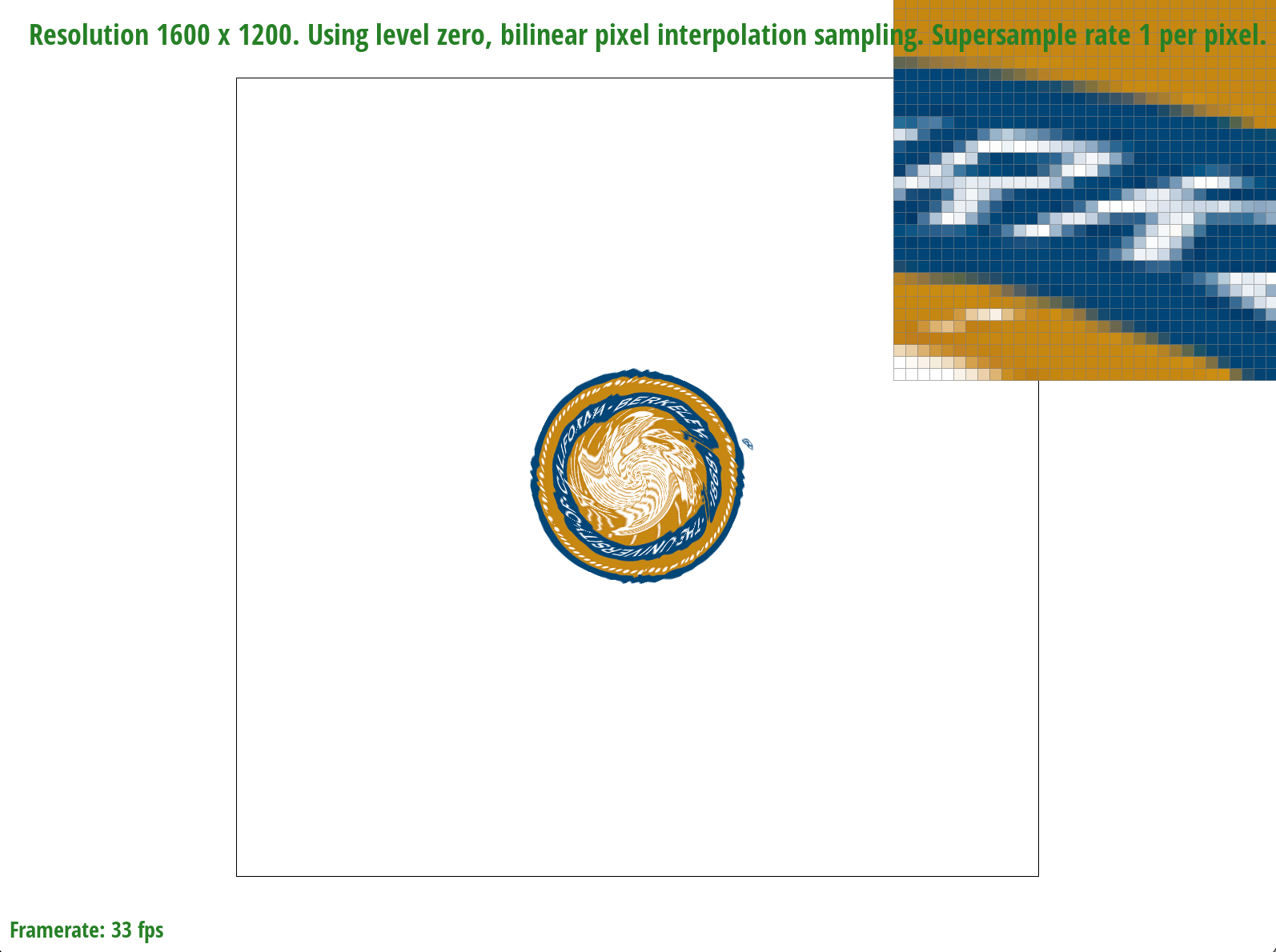
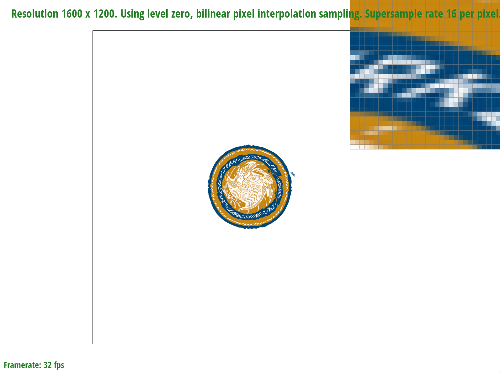
At lower sampling rates, the differences between the two methods are less obvious but as the sampling rate increases, bilinear sampling is generally better, especially when there are large variations in texel colors within a small area (ex: detailed textures) as pictured above. The nearest sampling at one sample per pixel is extremely pixelated in the magnified image but bilinear sampling "smoothens" this out even if we sample at one sample per pixel. Bilinear sampling at 16 samples per pixel is very "smooth" since the area is relatively small. We noticed that the largest difference between nearest and bilinear sampling is when there are significant changes in texel colors within a pixel. This makes sense because bilinear sampling will interpolate between texels whereas nearest sampling is unable to do so, potentially resulting in aliasing artifacts.
Task 6: "Level sampling" with Mipmaps for Texture Mapping
Implementation
Level sampling enables users to sample from textures with different precision levels. Mipmaps are a form of a low-pass filter to downsample the texture file, store the lower resolutions for each location then use it to downsample/minify the texture (ex: using multiple texture levels in a mipmap). In texture mapping, we generally want higher-resolution levels for areas with greater detail and lower-resolution levels for areas that require less sampling, thus enabling higher sampling and space efficiency. For example, we can use level zero image for close distances and use higher level image for further objects. Level sampling also allows us to estimate the texture footprint using coordinates of neighboring screen samples.
Nearest level sampling enables us to choose pixel by pixel which texture level to use to color, ideally, a 1:1 pixel to texel mapping. To implement nearest level sampling, we used the formula presented during lecture to compute the appropriate mipmap level to access. Afterwards, we scaled the uv texture coordinates to that level's resolution. Finally, we obtained the sample for the texture from that mipmap's level. For nearest sampling, it rounds the texel coordinates to the nearest integer.
Bilinear level sampling enables us to sample two different mipmap levels. We linearly interpolate between the two results based on where the "ideal level" would be - we calculate an "ideal" level and interpolate between the two closest integer levels surrounding the ideal. The level closer to the ideal level gets more weight which is then used to obtain the sampled texel color. For bilinear sampling, it calculates the fractional parts of the texel coordinates and performs bilinear interpolation between the texels.
get_level() was used often to determine the appropriate mipmap level based on the texture coordinates and the level sampling method. Notably, we needed to compute the difference vectors between texture coordinates and their partial derivatives inside this function instead of within the rasterize.cpp file, otherwise this would cause aliasing artifacts. Depending on the pixel sampling method (sp.psm), this determines what sampling function to call.
When comparing the three sampling techniques, pixel and level sampling both "smoothen" the pixels but supersampling takes exponential runtime memory. Bilinear sampling is CPU intensive since it uses four pixels around the sampling point. Level sampling is also CPU intensive because we need to calculate \((\frac{du}{dx}\), \(\frac{dv}{dx})\) and \((\frac{du}{dy}\), \(\frac{dv}{dy})\) to obtain the optimal mipmap level. Level sampling also has improved rendering speed compared to the other techniques, especially with large textures, because it chooses the appropriate mipmap level based on the texture's size and orientation, reducing the number of texels that need to be sampled.
Using the mipmap means that there is more memory overhead (an additional \(\frac{1}{3}\) storage space proportional to storing level 0), but this is generally okay since mipmaps have performance benefits (achieve coordinate-relative antialising at the cost of approx \(\frac{1}{3}\) more memory and 4 times texture reading time). The more we sample, the more time it takes to render the images. Level sampling also requires storing multiple versions of the texture at different resolutions, increasing memory usage compared to nearest or bilinear sampling (only requires original texture).
L_ZERO and P_NEAREST

L_ZERO and P_LINEAR

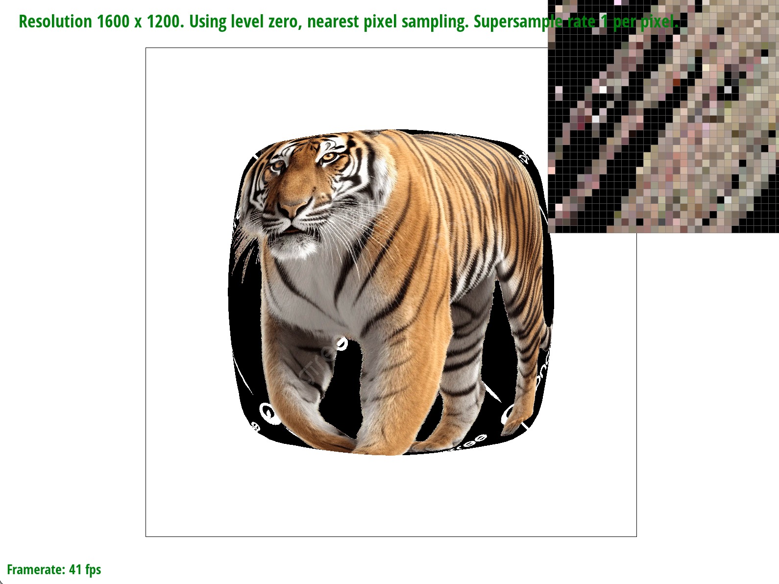
L_NEAREST and P_NEAREST
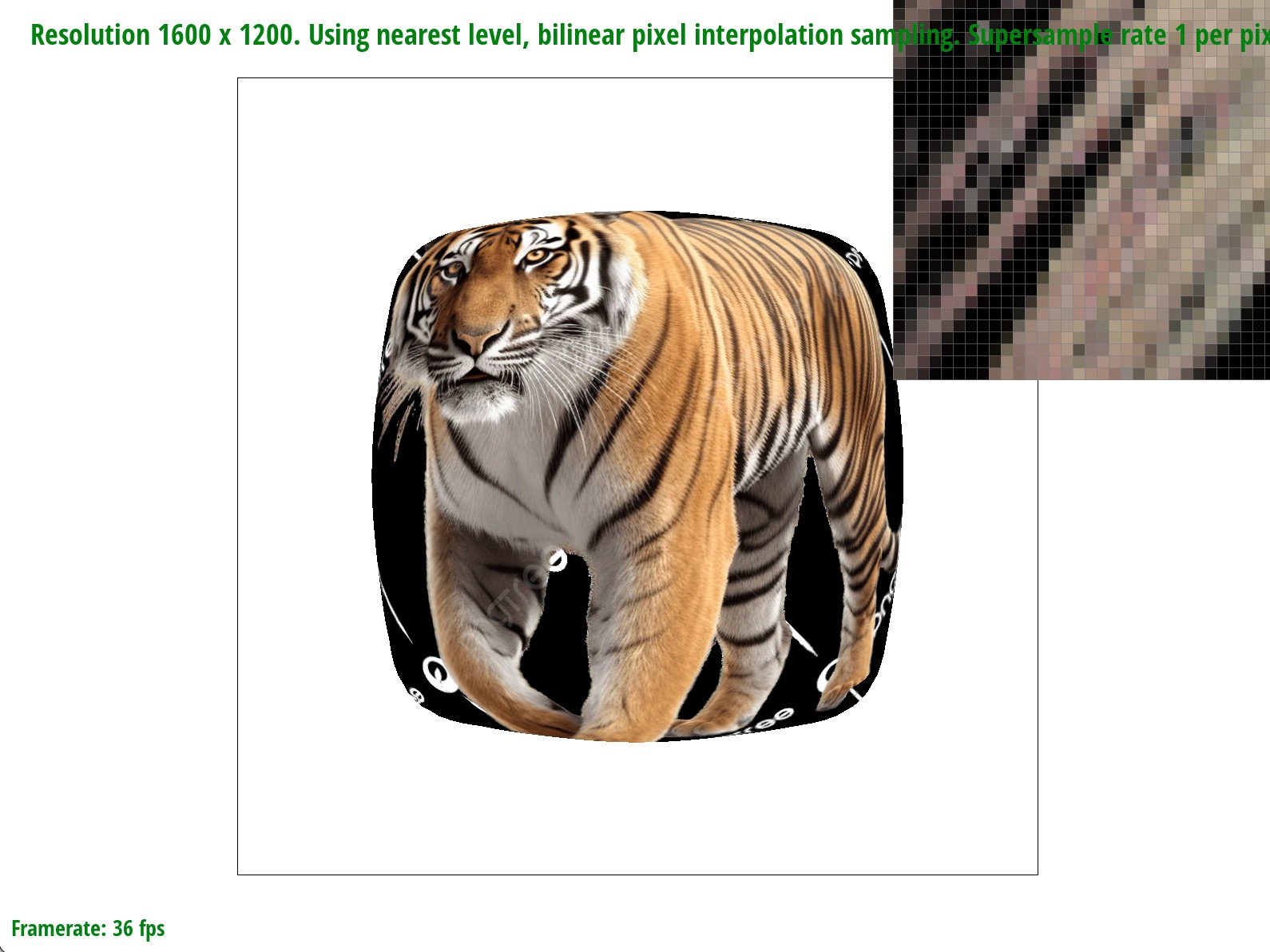
L_NEAREST and P_LINEAR