Overview
Site: https://cal-cs184-student.github.io/hw-webpages-sp24-christyquang/hw2/index.html
In this project, we build Bezier curves and surfaces using algorithms such as the de Casteljau algorithm. We also implememt features to manipulate give triangle meshes using the half-edge data structure. These features include performing edge splitting and edge flipping, which ultimately allows us to implement loop subdivision. This is quite an important feature for geometric 3D modeling, as it allows the artist to smoothen their meshes, as well as make them more detailed and customized to their liking. Being able to edit meshes after their original creation provides ease of modeling and being able to make small edits with the mesh. Focusing on the Bezier curves and surfaces themselves, implementing these features allows us to understand exactly how curvature is able to be simulated in a realistic way. Creating Bezier curves and surfaces allows us to create meshes in the first place, which we can then use to model 3D objects and edit the meshes with the functions described earlier.
We found it particularly interesting how the assignment builds on each other, and allows full understanding of what lays underneath geometric modeling. First, we build the actual Bezier curves and surfaces, then we build implementation to edit these curves and meshes to our liking. It was especially interesting navigating the half-edge data structure. Although a bit complicated at first, the different parameters and built-in functions proved to be extremely useful when working with the meshes. It allowed for easy access to the different parts of the mesh, so that we could edit only exactly what we needed to edit without a lot of overhead.
Section I: Bezier Curves and Surfaces
Part 1: Bezier curves with 1D de Casteljau subdivision
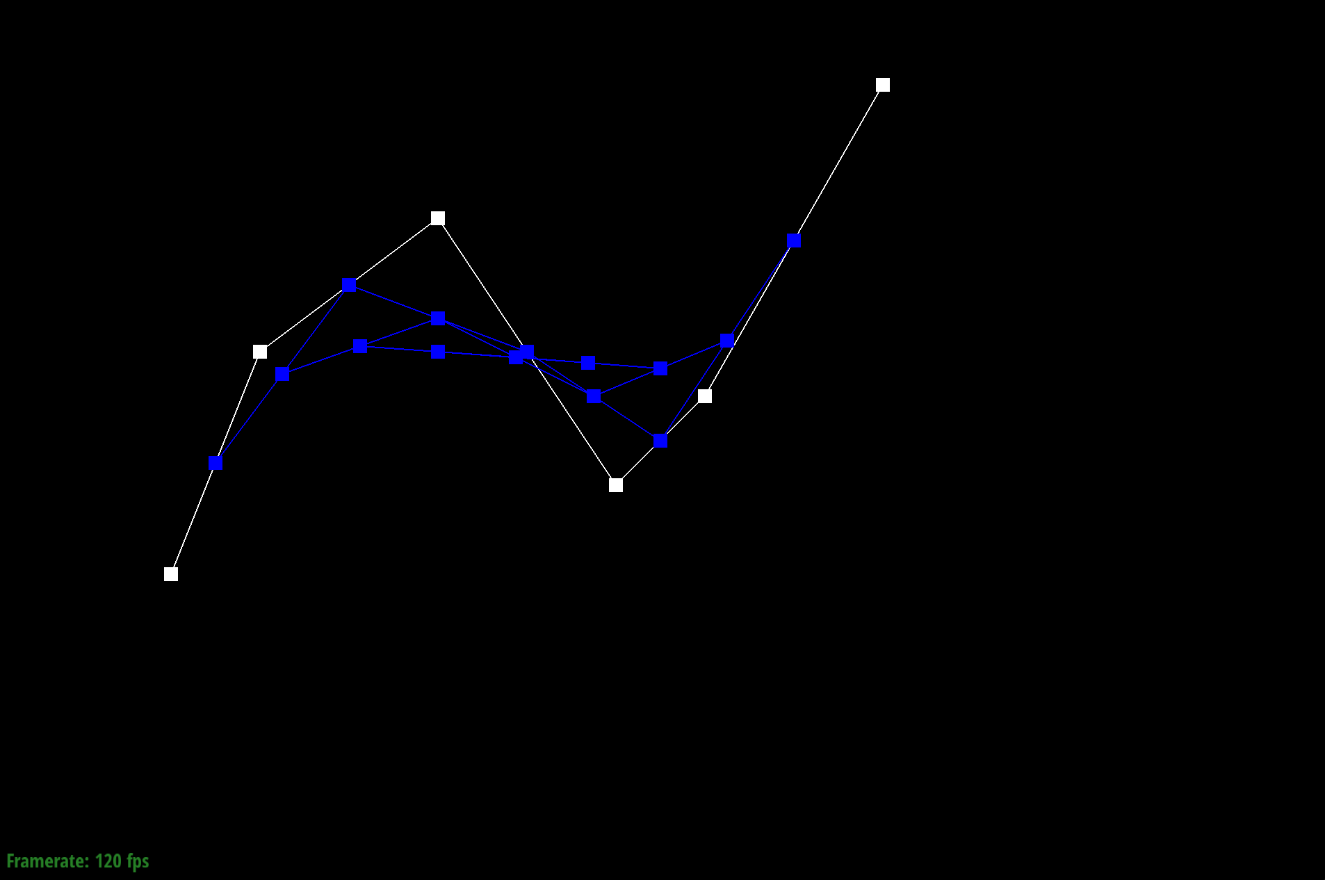
de Casteljau's algorithm is a recursive method that allows us to calculate a Bezier curve from a set of points. Given n control points, we recursively subdivide the n-1 line segments between the control points and define interpolated points. The process involves connecting the points to create edges, then we evaluate each edge at a parameter t which is between 0 and 1, representing a fraction of the distance from one point to the other point. For example, we can have points x0 and x1, where point x01 is along the line from x0. Since t determines our location between the points, when t = 0, we are at x0. We connect the points to get a connection of edges that is one less than the previous number of edges. We recursively interpolate points until we run out of line segments (keep creating line segments between adjacent interpolated points and put a new interpolated point on that line segment). The final point we arrive at is a point on the Bezier curve at the given parameter t.
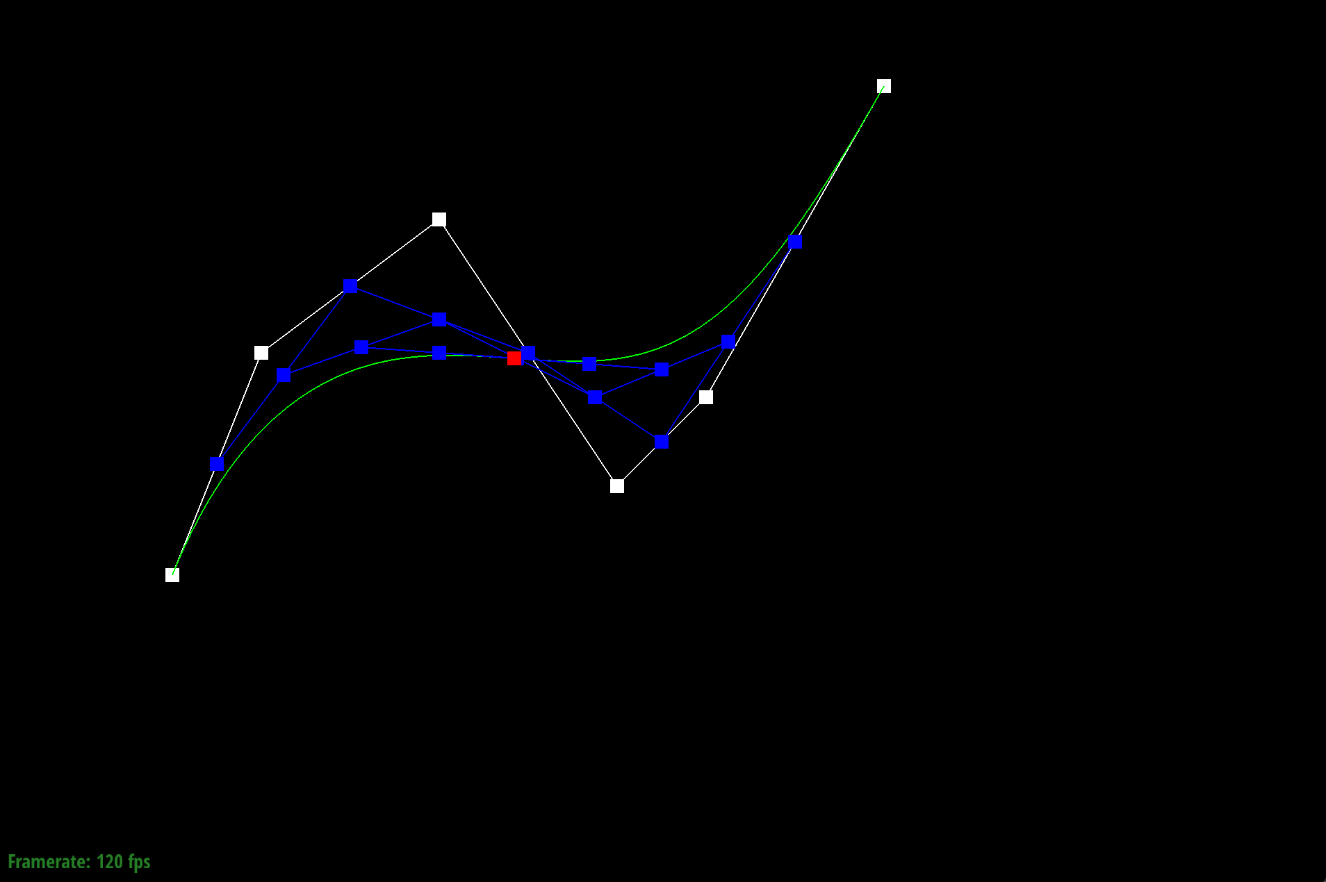
We implemented evaluateStep which performs one step of the algorithm (or one level of subdivision) each time it is called. First, we obtain the size of the most recent level using points.size(). If the level is 1, we can just return points. Otherwise, we use the algebraic formula $$p_i' = \text{lerp}(p_i, p_{i+1}, t) = (1 - t)p_i + tp_{i+1}$$ to find the interpolated point between each pair of adjacenet points up to the most recent level (numPoints - 1), enabling us to get to the last evaluated point.
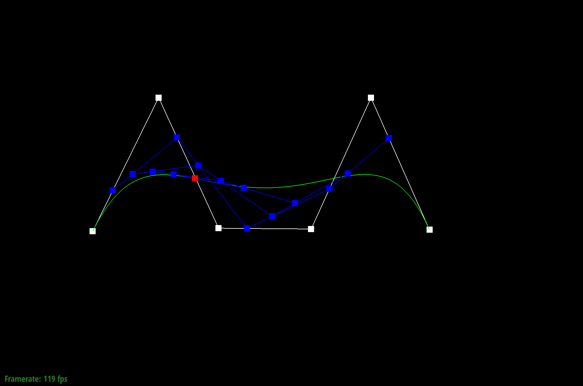
Below are screenshots of each step of the evaluation from the original control points down to the final evaluated point.
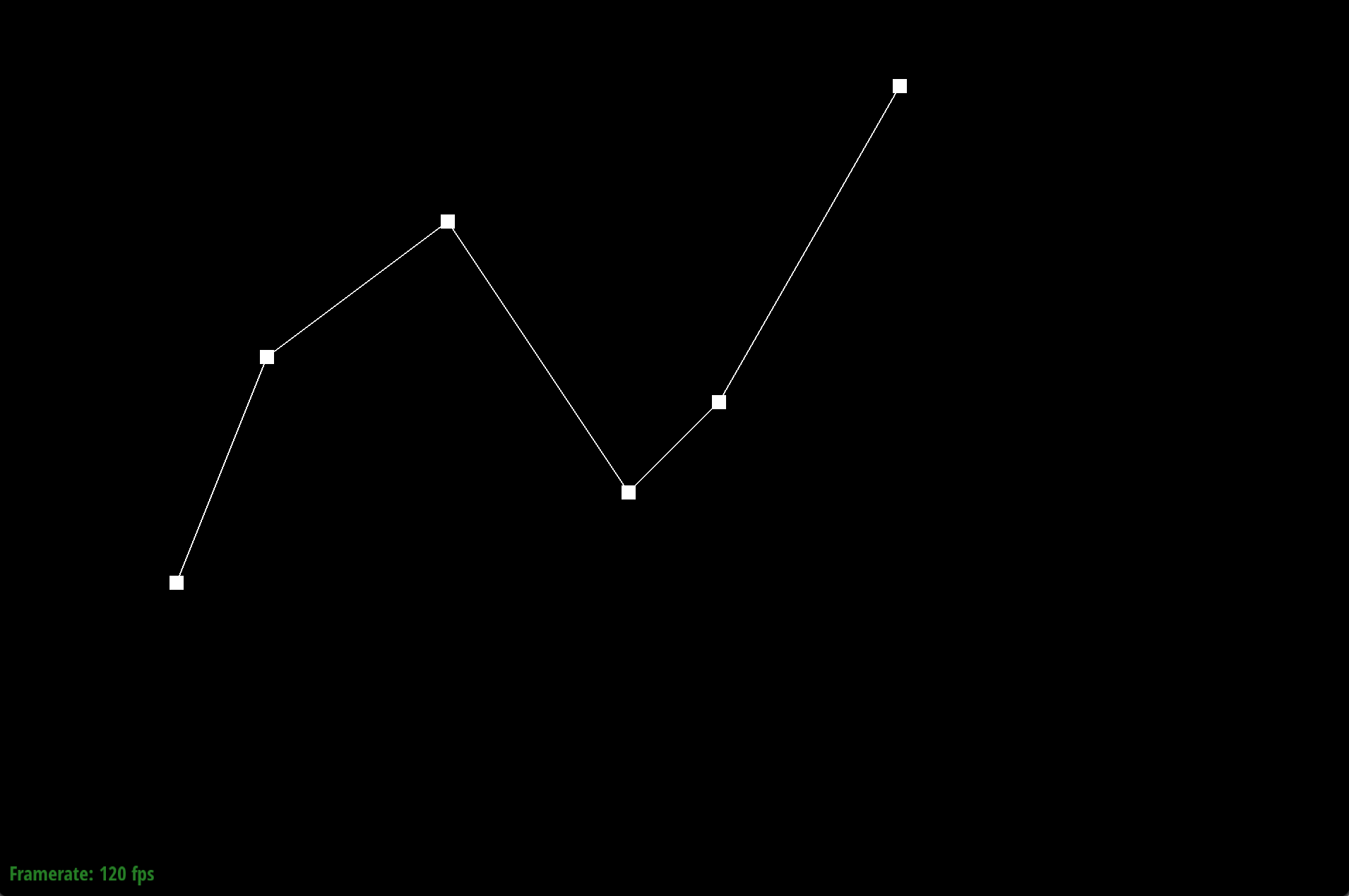
Original control points
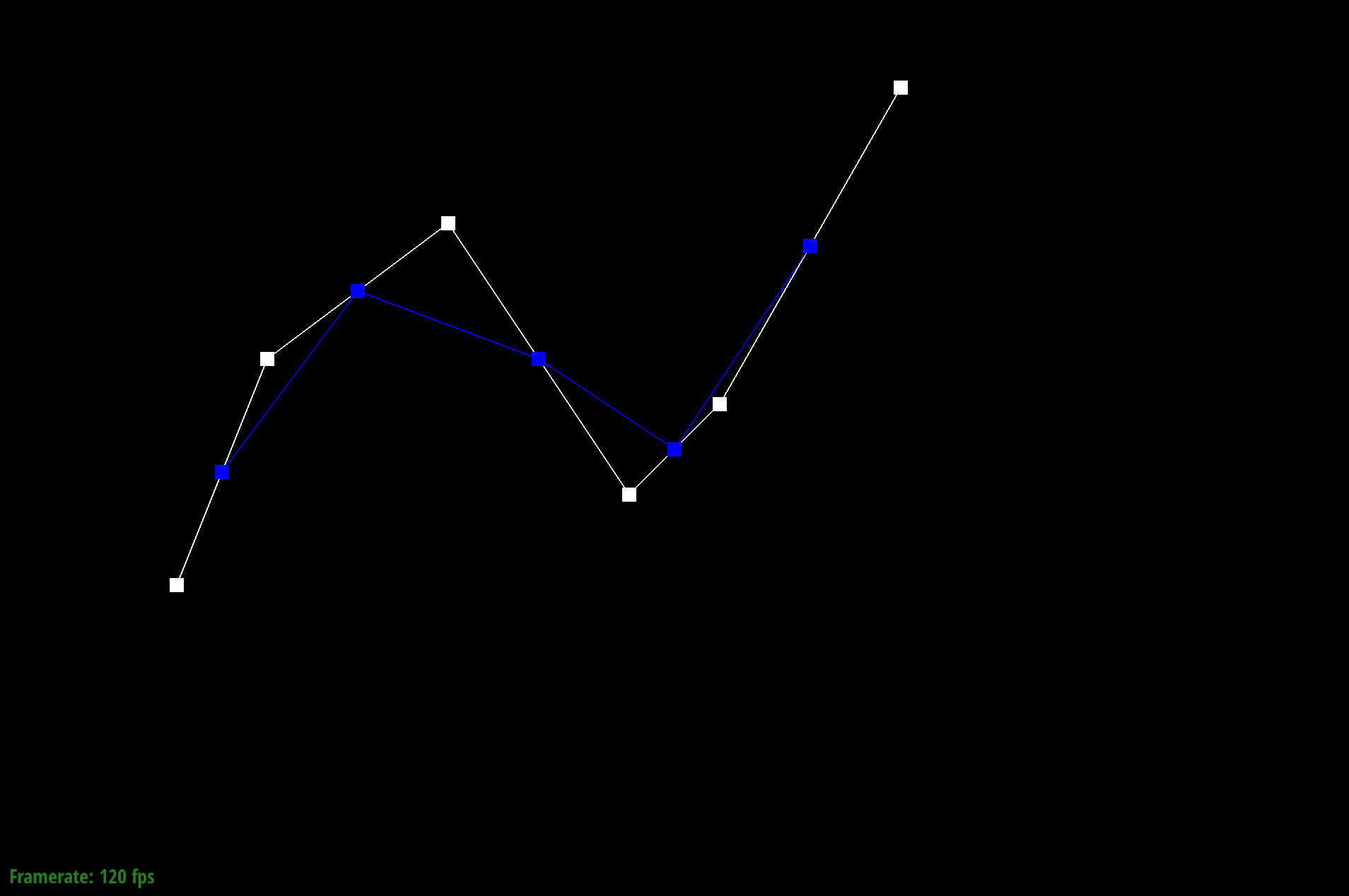
Bezier curve Step 1
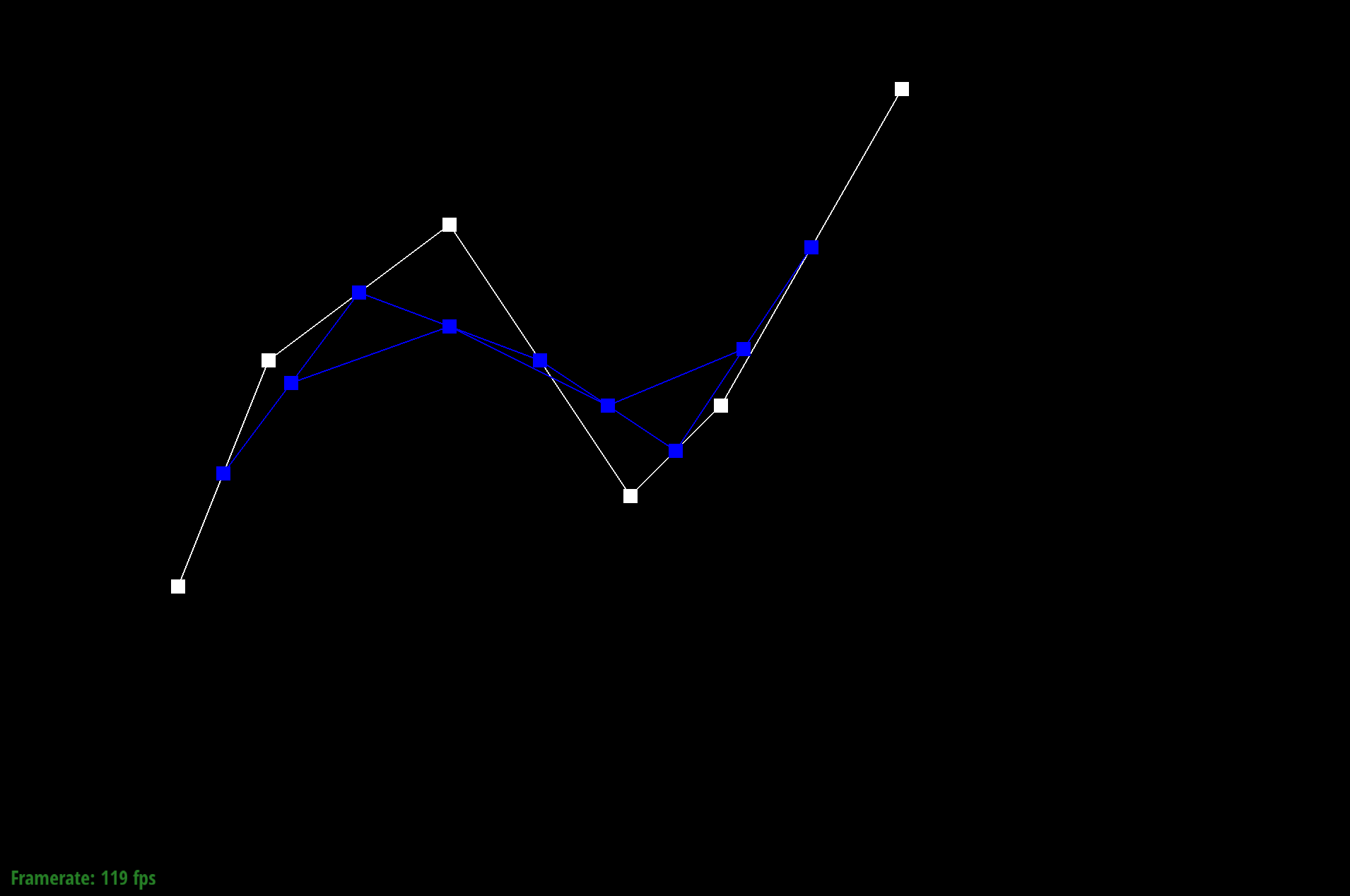
Bezier curve Step 2
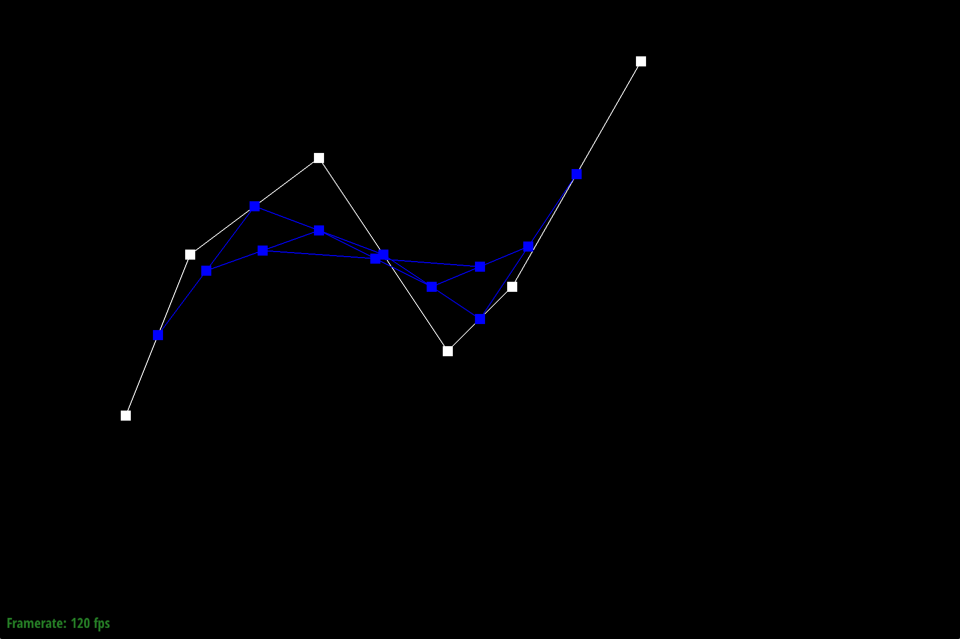
Bezier curve Step 3
Bezier curve Step 4
Bezier curve Step 5
Here’s the completed Bezier curve created from running de Casteljau’s algorithm above.
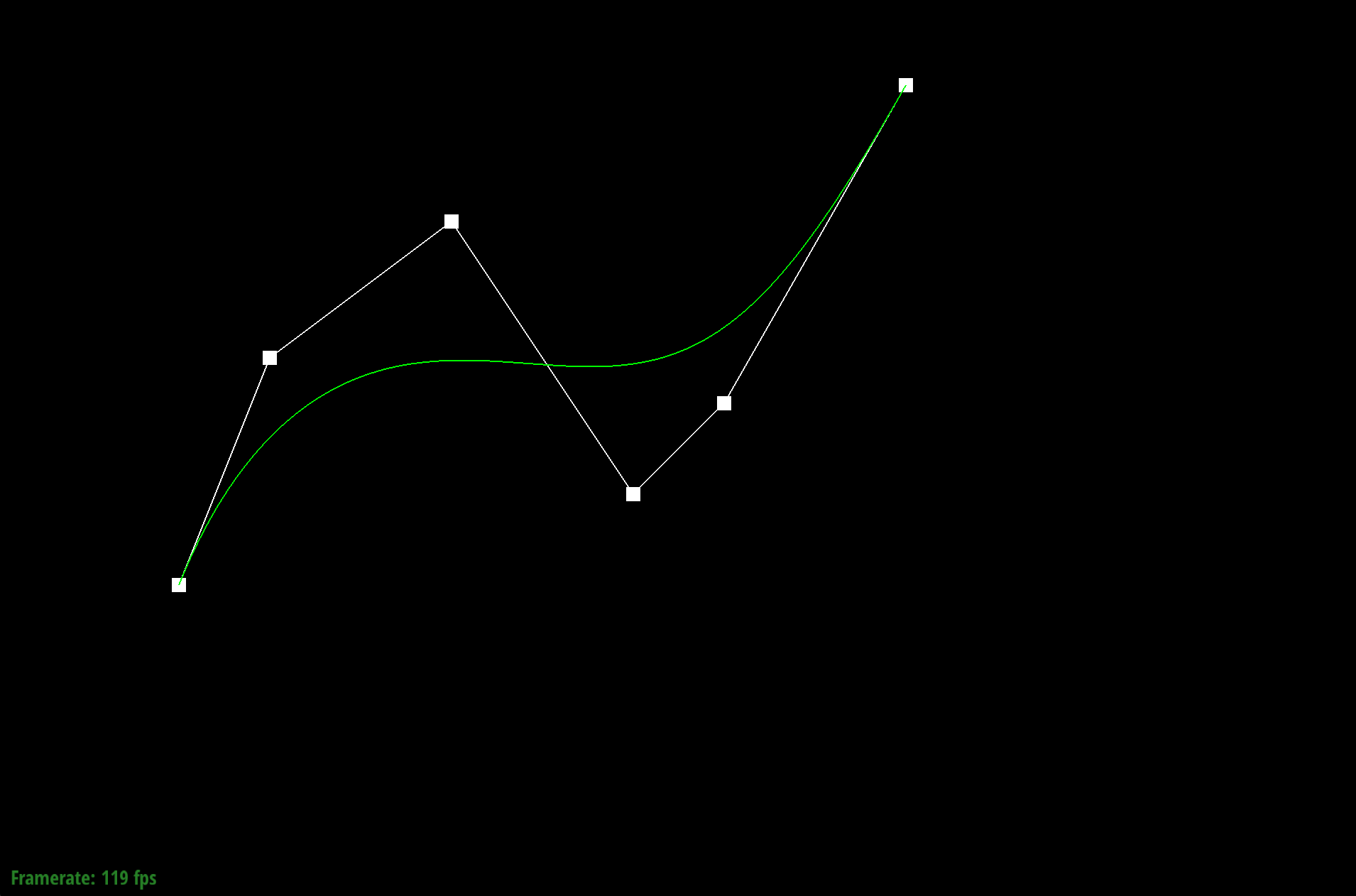
Completed Bezier curve
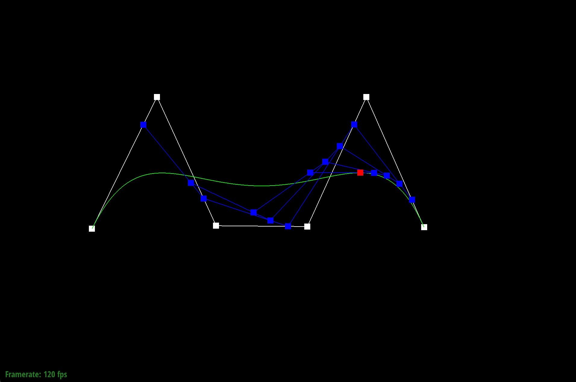
We can also drag and move the original control points to create a new Bezier curve. Below is an example of a modified Bezier curve we've created.
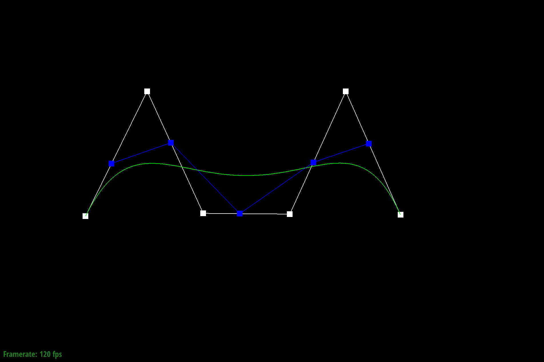
Different Bezier curve
Lastly, we are able to modify the parameter t to show the other points lie along the completed green Bezier curve.
Different Bezier curve and lower t value
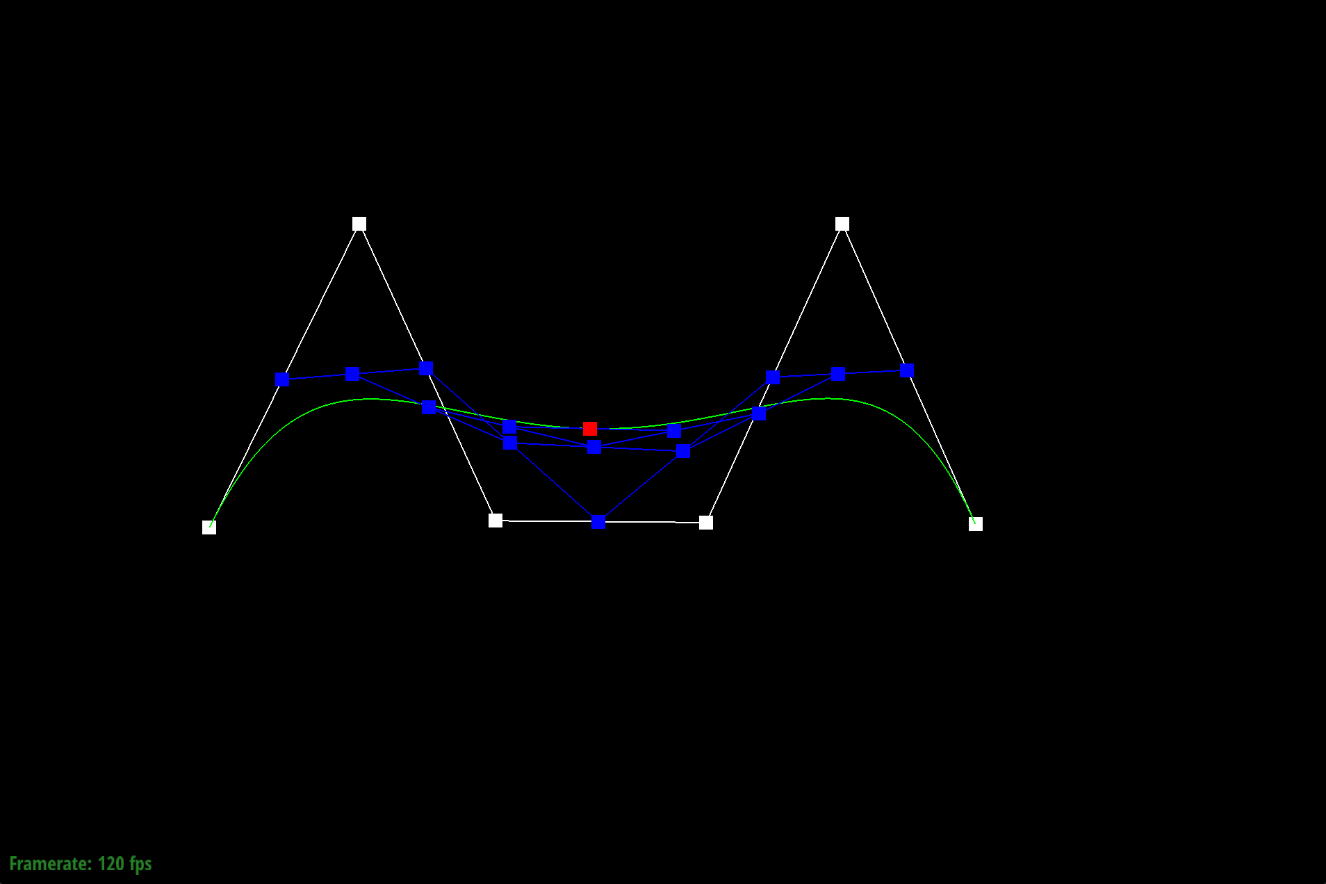
Different Bezier curve and slightly increasing t value
Different Bezier curve and greatest increasing t value
Part 2: Bezier surfaces with separable 1D de Casteljau
The de Casteljau algorithm extends to Bezier surfaces because we are able to apply the same process we did for the 1 dimensional curve to a 2 dimensional curve by adding another dimension. Applying multiple Bezier curves together creates a Bezier surface. In Part 1, we had n control points to define a Bezier curve but in Part 2, we had a matrix of n x n control points to define a Bezier curve. We perform the 1D de Casteljau algorithm on each row to get one point per row for each u via calling the evaluate1D function repeatedly. Then, we performed the algorithm and interpolation again on the points to get the final point in the v direction, resulting in one point that lies on the Bezier surface at the given u and v.
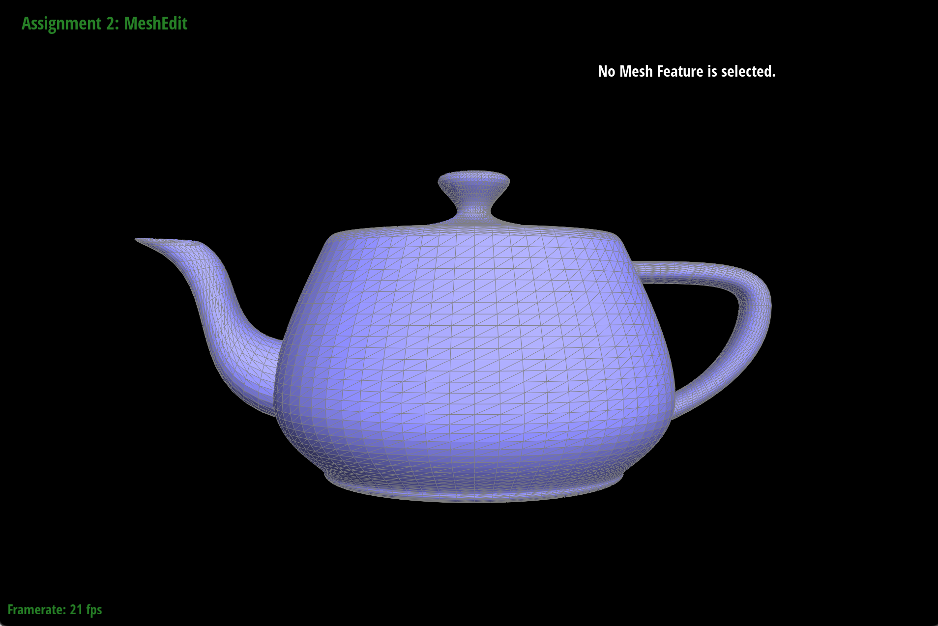
Screenshot of bez/teapot.bez
Section II: Triangle Meshes and Half-Edge Data Structure
Part 3: Area-weighted vertex normals
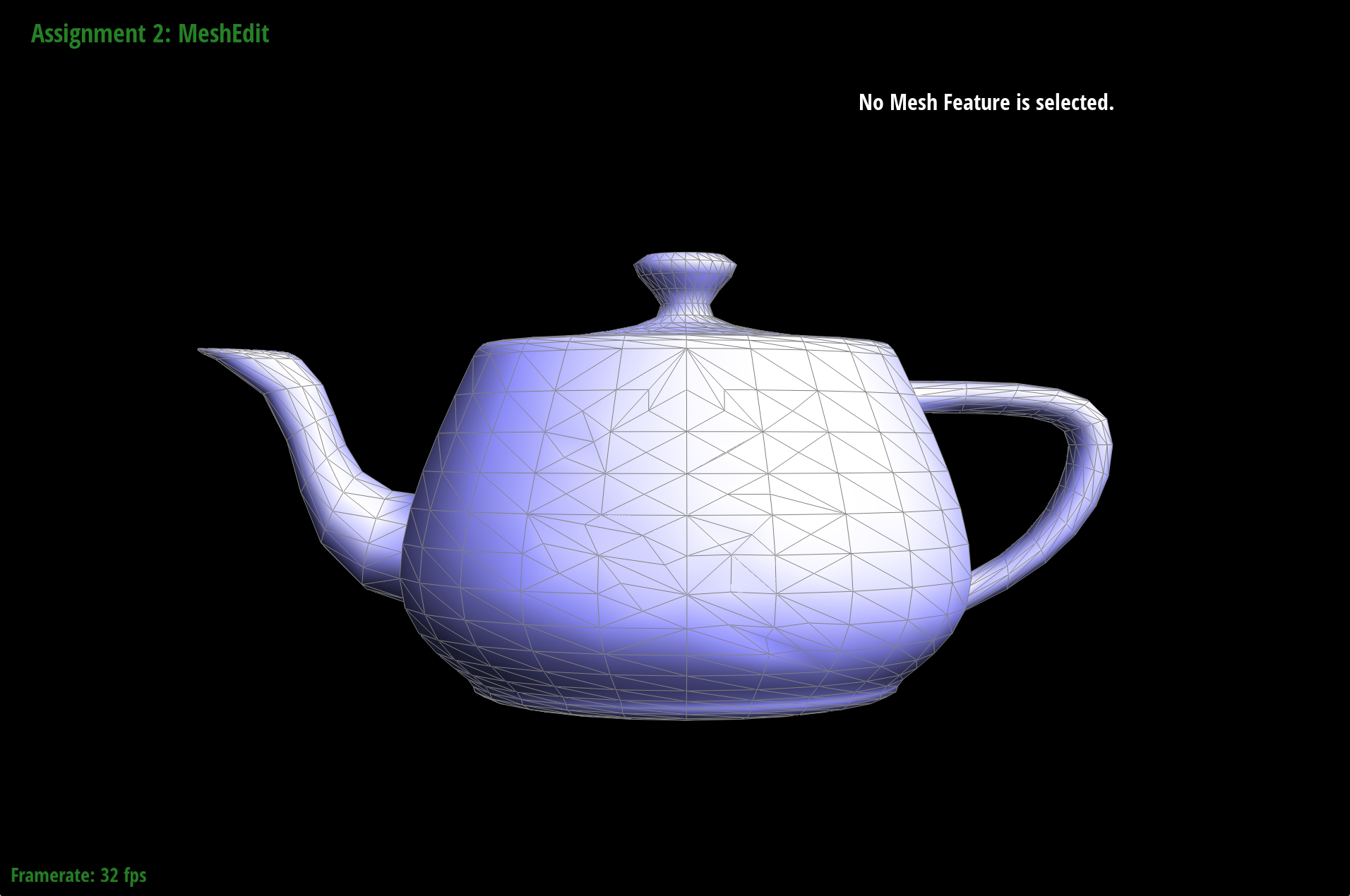
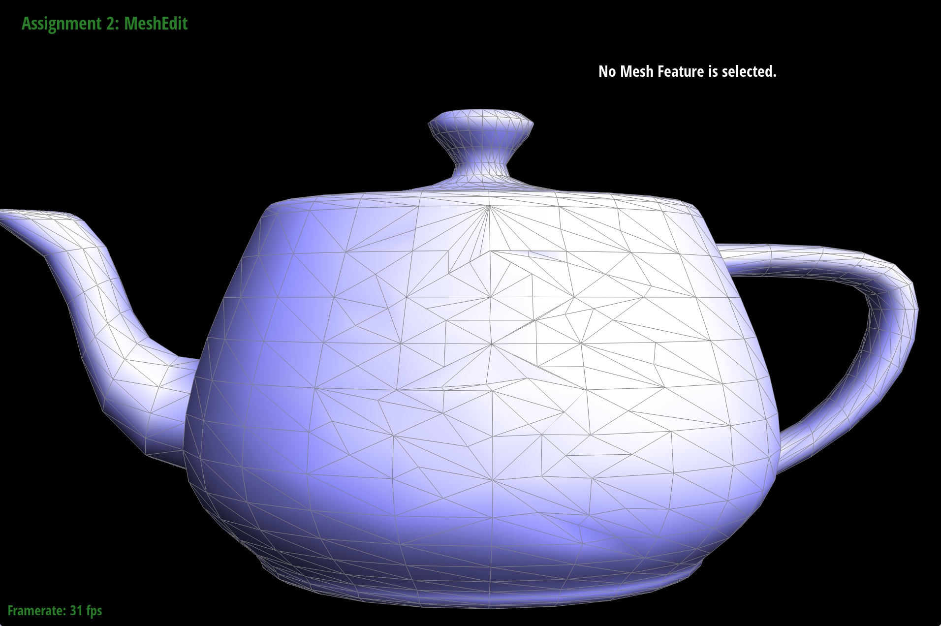
We implemented the area-weighted vertex normals by iterating through all the triangles incident to the vertex (faces that have the given vertex as one of the vertices), allowing us to have smoother shading on dae/teapot.dae. First, we iterated through the half-edges incident to the vertex h. Inside the loop, we calculate the normal vector of each triangle incident to the vertex. We found the positions of three vertices: the current vertex (commonPoint) and two vertices connected to it through two consecutive half-edges. Then, we computed the vectors representing the sides of the triangle formed by the vertices. The normal of the triangle is calculated by taking the cross product of these two edges which is added to weightedNormal, accumulating the contributions from all of the triangles (gets the area-weighted normal of the face). After iterating through the faces, we return the re-normalized unit vector by calling weightedNormal.unit().
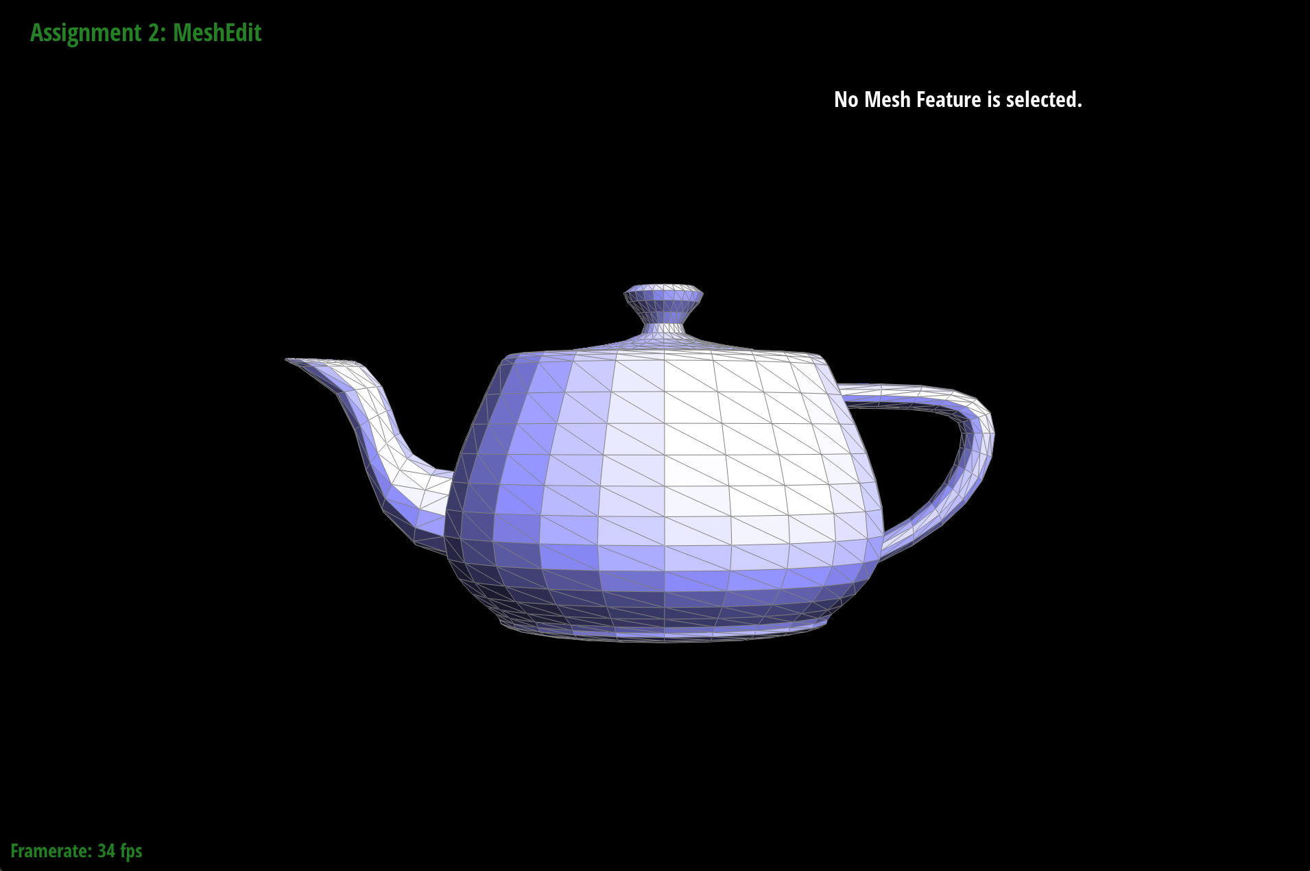
dae/teapot.dae without vertex normals (flat shading)
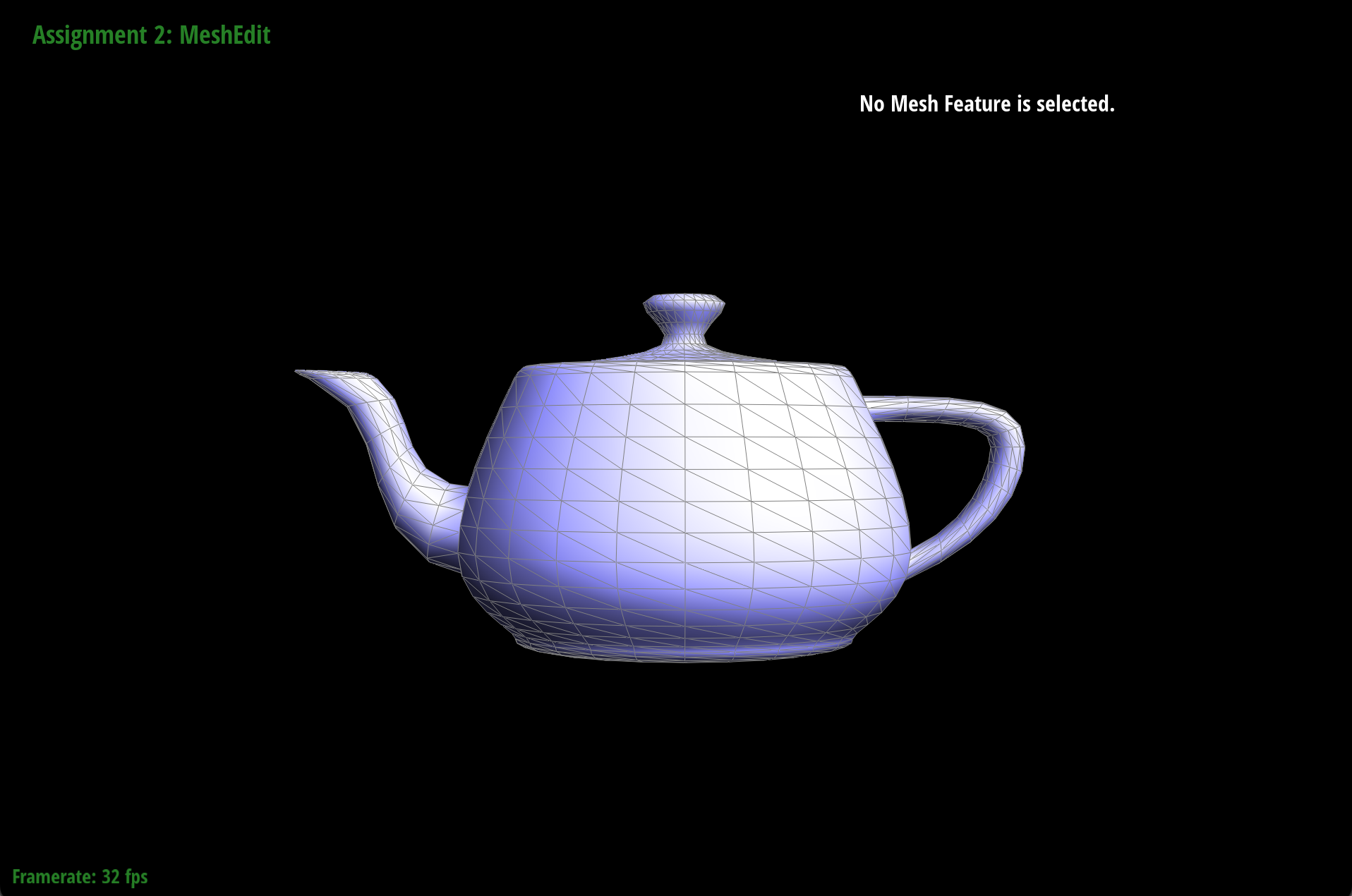
dae/teapot.dae with vertex normals (Phong shading)
Part 4: Edge flip
When there is an edge shared between two triangles, the edge flip operation changes the orientation such that the edge now spans across the other two corners of the triangles. To do this, we first kept track of all the mesh elements: half-edges, vertices, edges, or faces. The edge flip operation reassigns pointers to these elements so it's important to keep track of where each element changes to, otherwise it's very messy to implement. Before implementing the function, we drew out the before and after meshes of the edge flip, taking note of how each element changed.
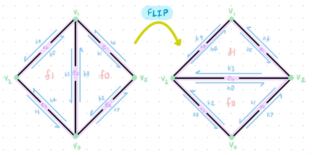
Screenshot of our brainstorming process when implementing the edge flip functionality
We had hoped that by doing this, it would save us a lot of debugging time since we were certain that the pointers were reassigned correctly. We created variables for every element starting with the half-edges and utilized the setNeighbors function on each half-edge to make sure that the neighboring elements were correctly assigned. Drawing the meshes was extremely helpful but I still spent a couple of hours debugging an extremely small bug where I had written HalfedgeIter h9 = h4->twin(); instead of HalfedgeIter h9 = h5->twin();. This caused edge flips to not work on certain edges on the teapot which would crash the program. Besides this terrible bug, the function was fun to implement and here are some screenshots displaying before/after an edge flip, as well as dae/teapot.dae after a series of cool edge flips.
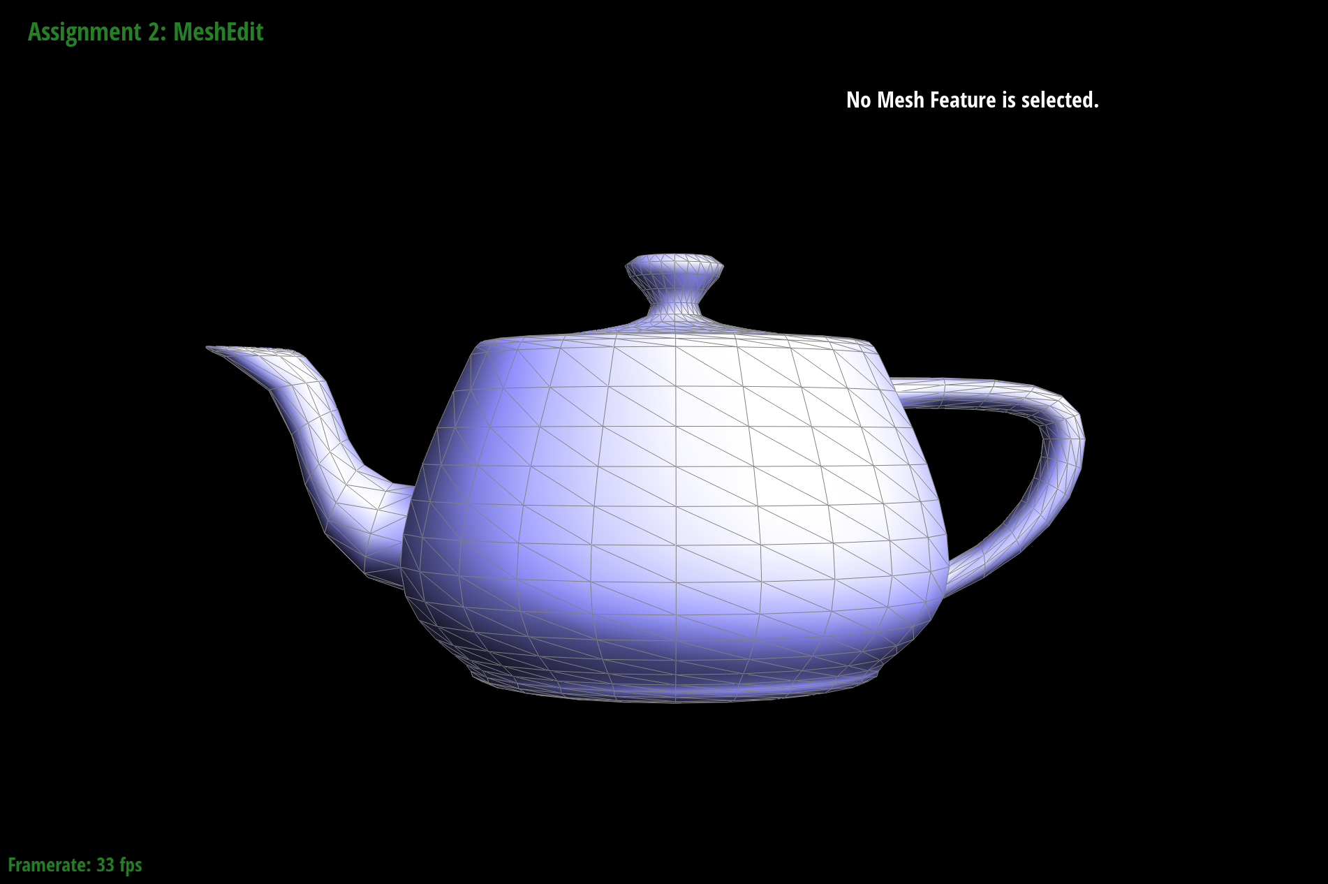
dae/teapot.dae before an edge flip

dae/teapot.dae after an edge flip
dae/teapot.dae with some cool edge flips
Part 5: Edge split
When there is an edge shared between two triangles, the edge split operation inserts a new vertex m at its midpoint and connects the new vertex to each opposing vertex that didn't previously have an edge connecting to them, creating four triangles from two adjacent triangles. This operation was similar to the edge flip operation but there were a few new components to keep track of since an edge split adds new mesh elements: a new vertex, two new triangles (six new half-edges), three new edges, and two new faces.
With all of the new elements being added, there are more pointers to keep track of than for the edge flip operation so we followed the same strategy of drawing out the before and after meshes of the edge split, taking note of how each element changed.
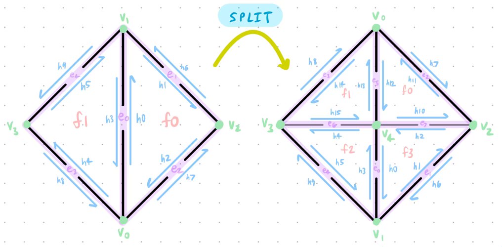
Screenshot of our brainstorming process when implementing the edge split functionality
Despite drawing the mesh after the edge split, it was significantly harder than the edge flip functionality because we had to decide where to put the new elements. We created variables for every element starting with the half-edges, and created new variables to represent the new elements being added. Similar to the edge flip method, we utilized the setNeighbors function on each half-edge to make sure that the neighboring elements were correctly assigned. With the new pointers being created/assigned, there are now four half-edge cycles instead of the previous two. As a result, I had to change the half-edges, vertices, edges, twins, and faces for a majority of the half-edges. The new vertex is just the middle distance between the two endpoints of edge e0. The diagram significantly helped me and made implementing this function mostly bug-free.
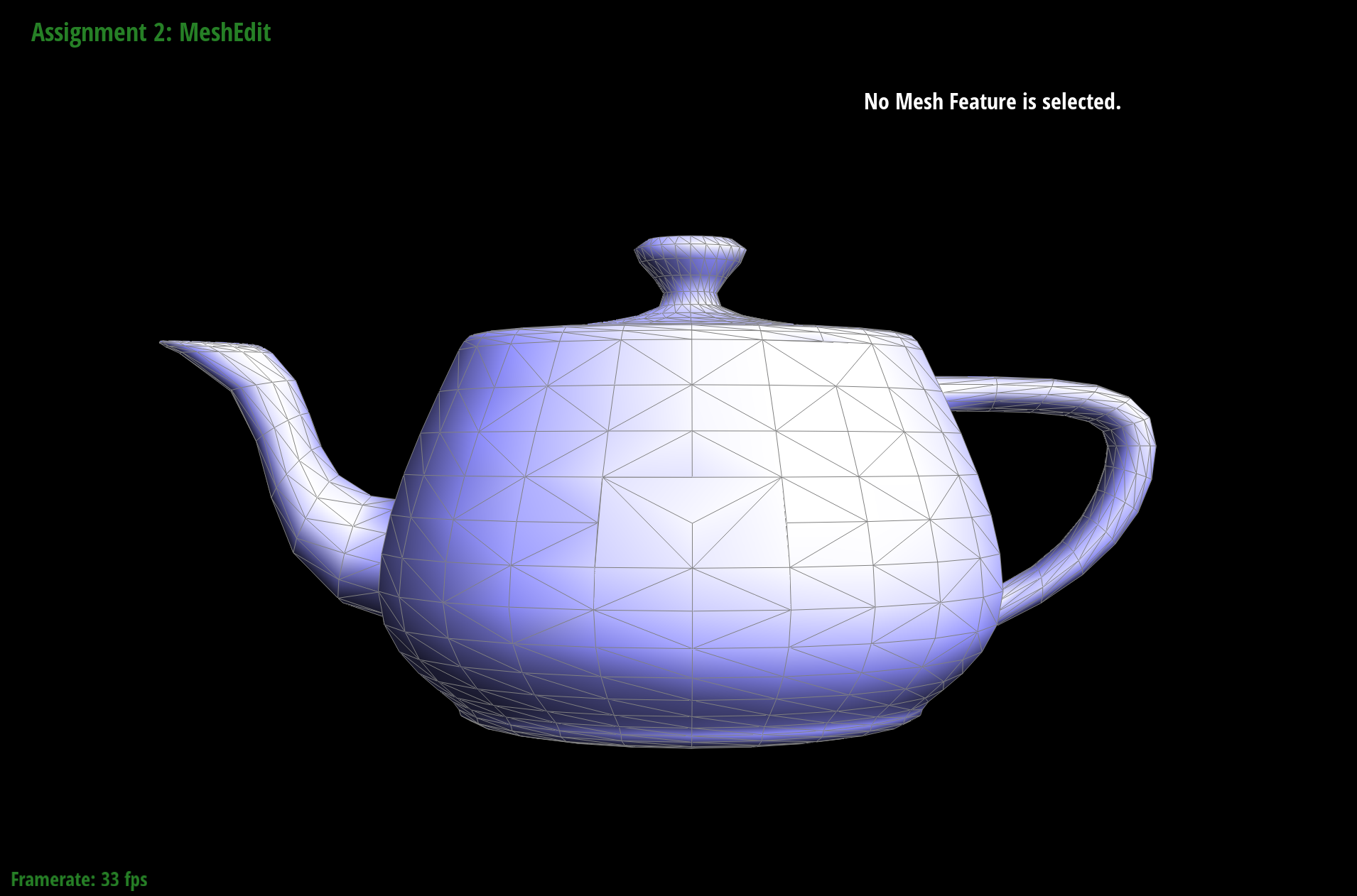
dae/teapot.dae before an edge split
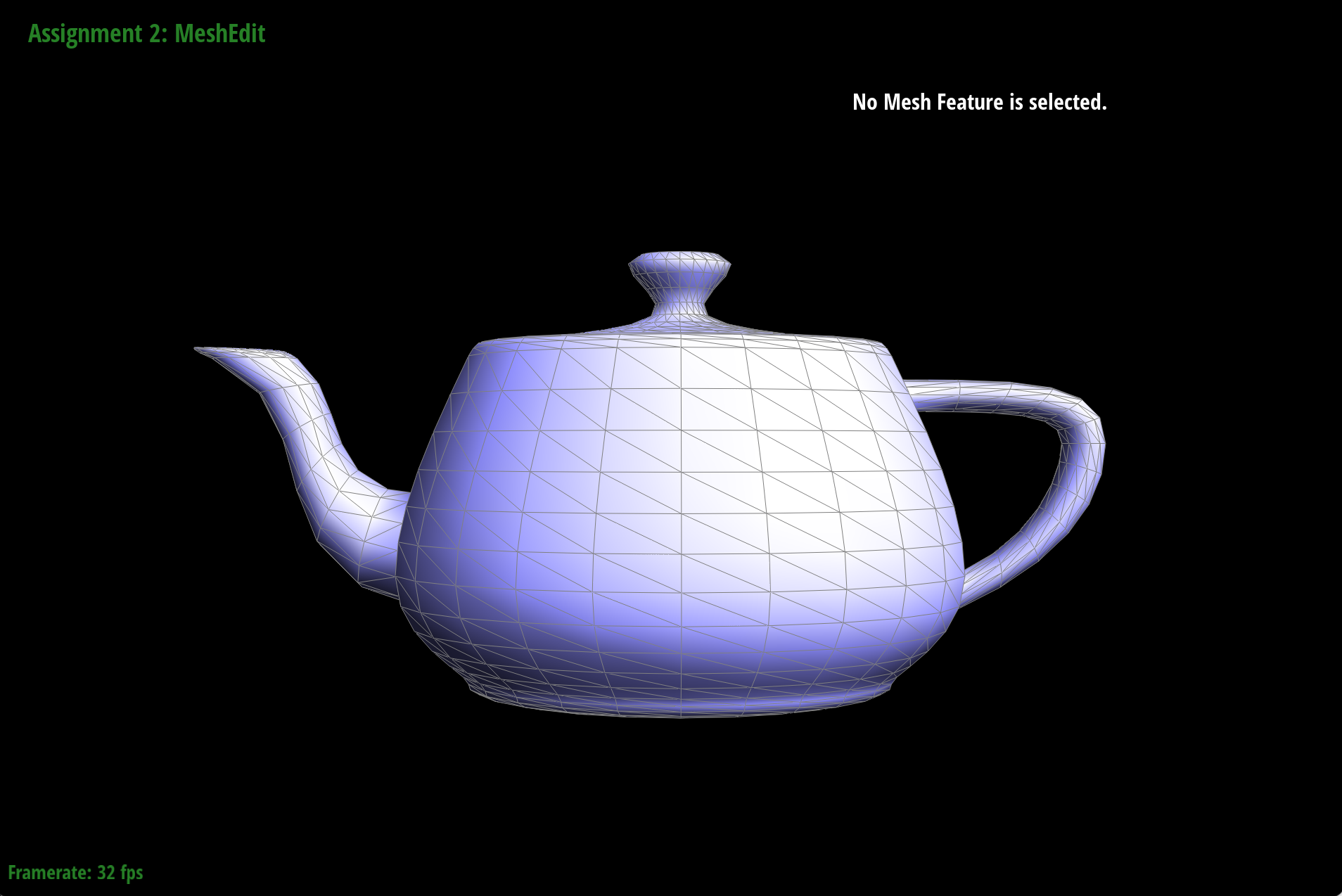
dae/teapot.dae after an edge split
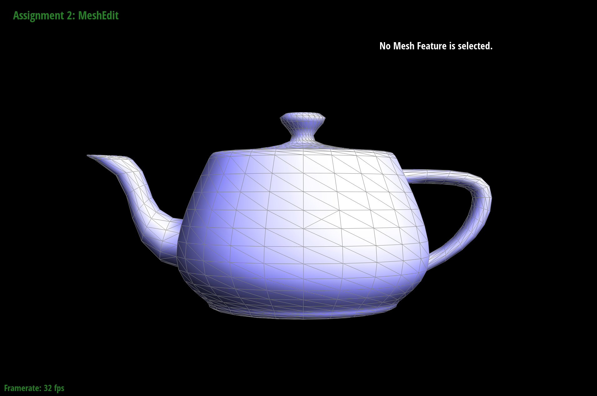
Part 1: dae/teapot.dae after some cool edge splits and flips
Part 2: dae/teapot.dae after some cool edge splits and flips
Part 6: Loop subdivision for mesh upsampling
To implement loop subdivision, we mainly followed the steps given in the spec and in the function definition. First, we computed all the new positions of the original vertices, as well as the position of the new vertices created by edge splitting. This involved iterating through all the vertices in the edge, finding the halfedges and calculating the sum of the positions of the adjacent vertices. Specifically, the new position was calculated by v->newPosition = (1.0 - n * u) * v->position + u * weighted_sum;. n represented the number of edges incident to the vertex and u = 3/16 if n = 3, otherwise 3/(8n). weightedSum represented the sum of all the original positions of neighboring vertices.
To compute the new positions, we traversed through the edges and for each edge, we found the surrounding edges and vertices and calculated e->newPosition = (3.0/8.0) * (v0->position + v1->position) + (1.0/8.0) * (v2->position + v3->position);. v0 and v1 represented the two vertices connecting the current edge. Then, we actually split the edge, making sure to only split the original edges and not the newly added edges.
Afterwards, we flip certain edges, being careful that we are only flipping those that connect a new and old vertex, and are also newly added edges. This was done by iterating through all the edges and flipping them by connecting an old vertex to a new one.
Finally, we actually update the vertex positions with the values that were calculated earlier by copying their newPosition into their position attribute. One very key and interesting implementation trick we used is incorporating the isNew flag for vertices and edges, helping us ensure that we were only splitting and flipping the edges that we need to. This involved going back to the previous functions, specifically splitEdge, and setting the isNew flag whenever we created a new vertex or edge.
It seems that after loop subdivision, the sharp corners and edges are smoothened out. They become more round, as shown in these pictures below because we are increasing the number of triangles, allowing for more smooth curves to develop.
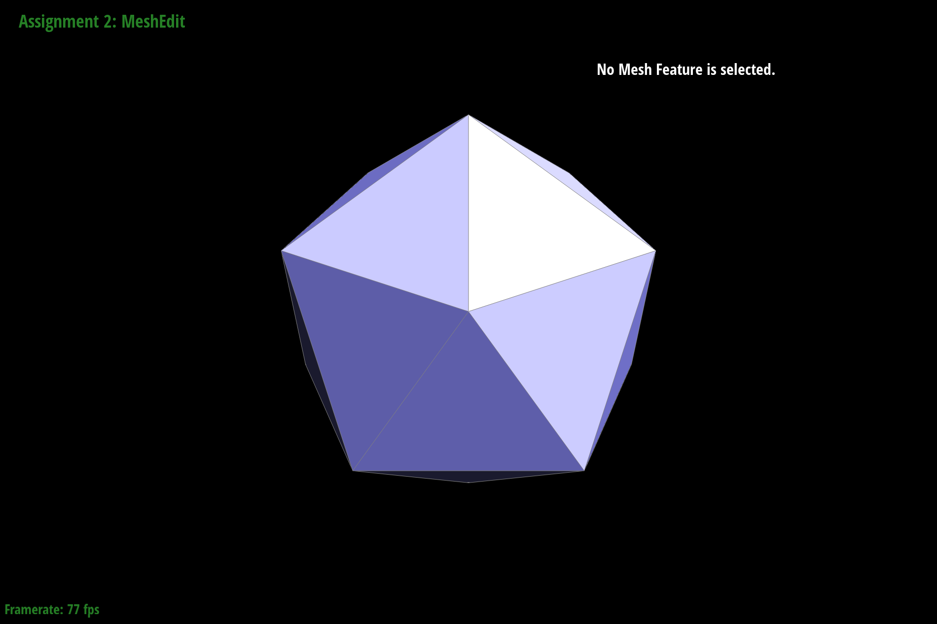
Icosahedron Loop Subdivision 1
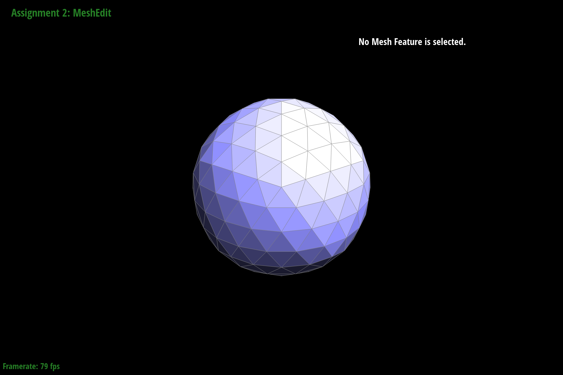
Icosahedron Loop Subdivision 2
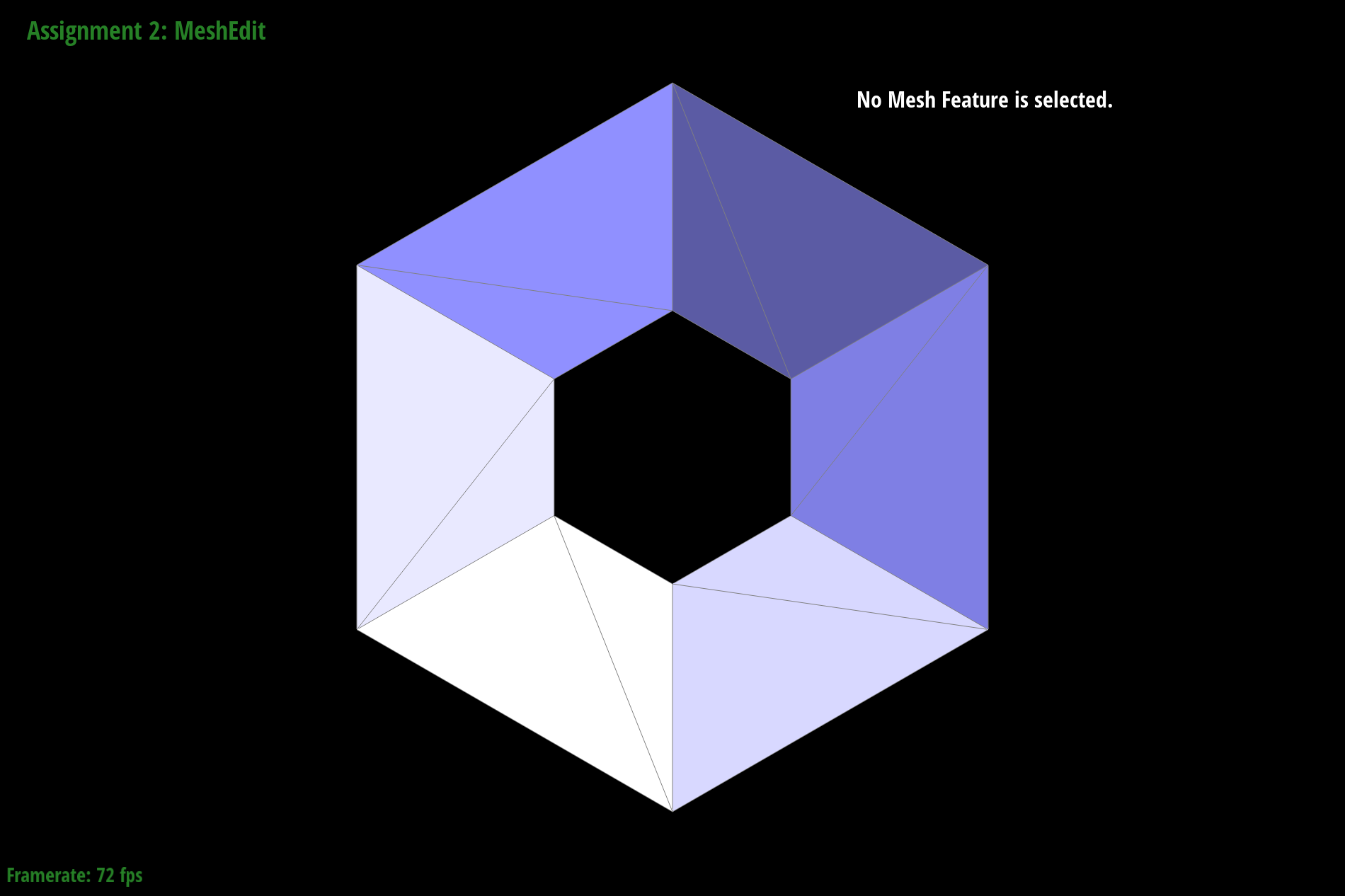
Torus Loop Subdivision 1
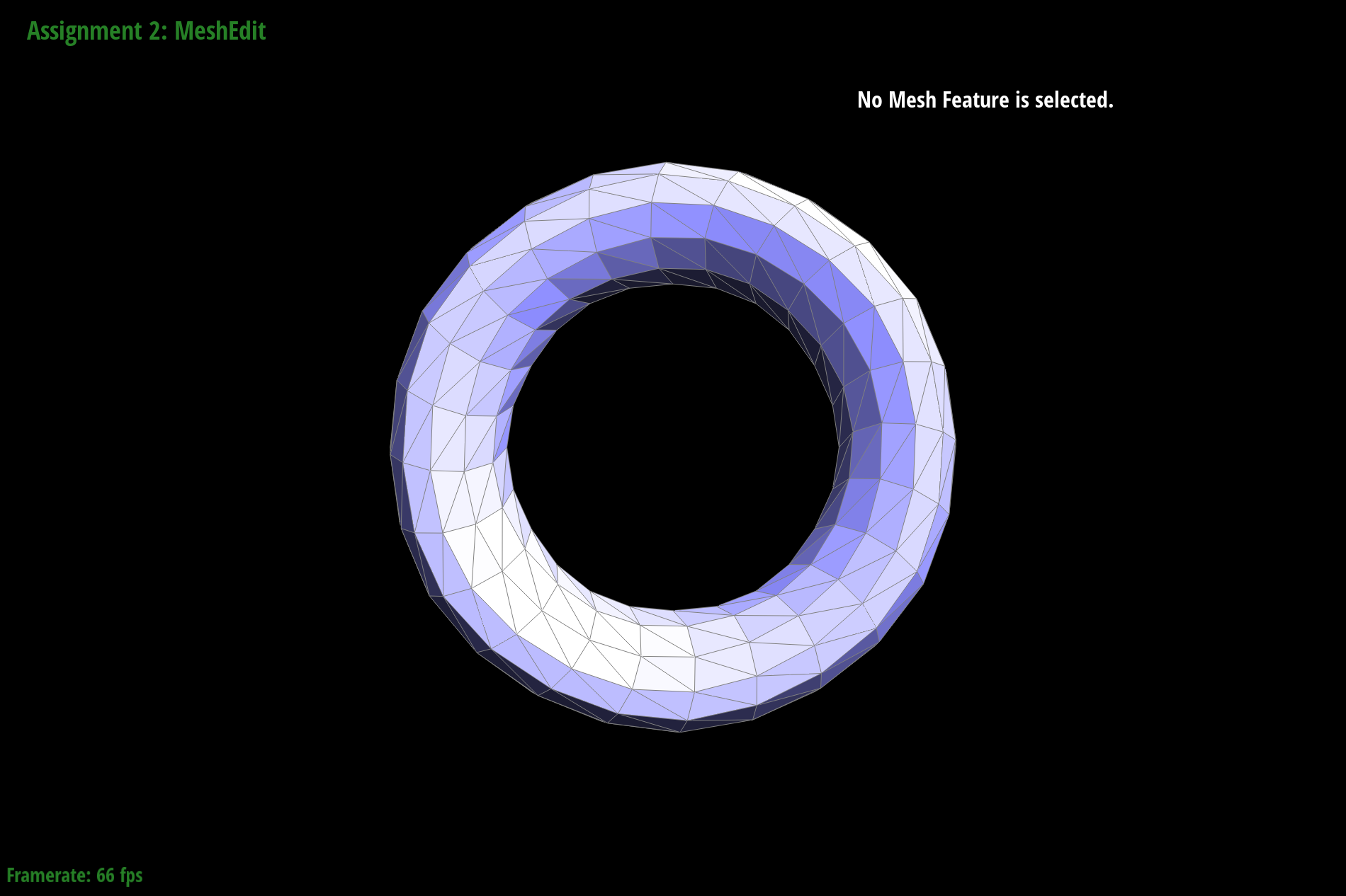
Torus Loop Subdivision 2
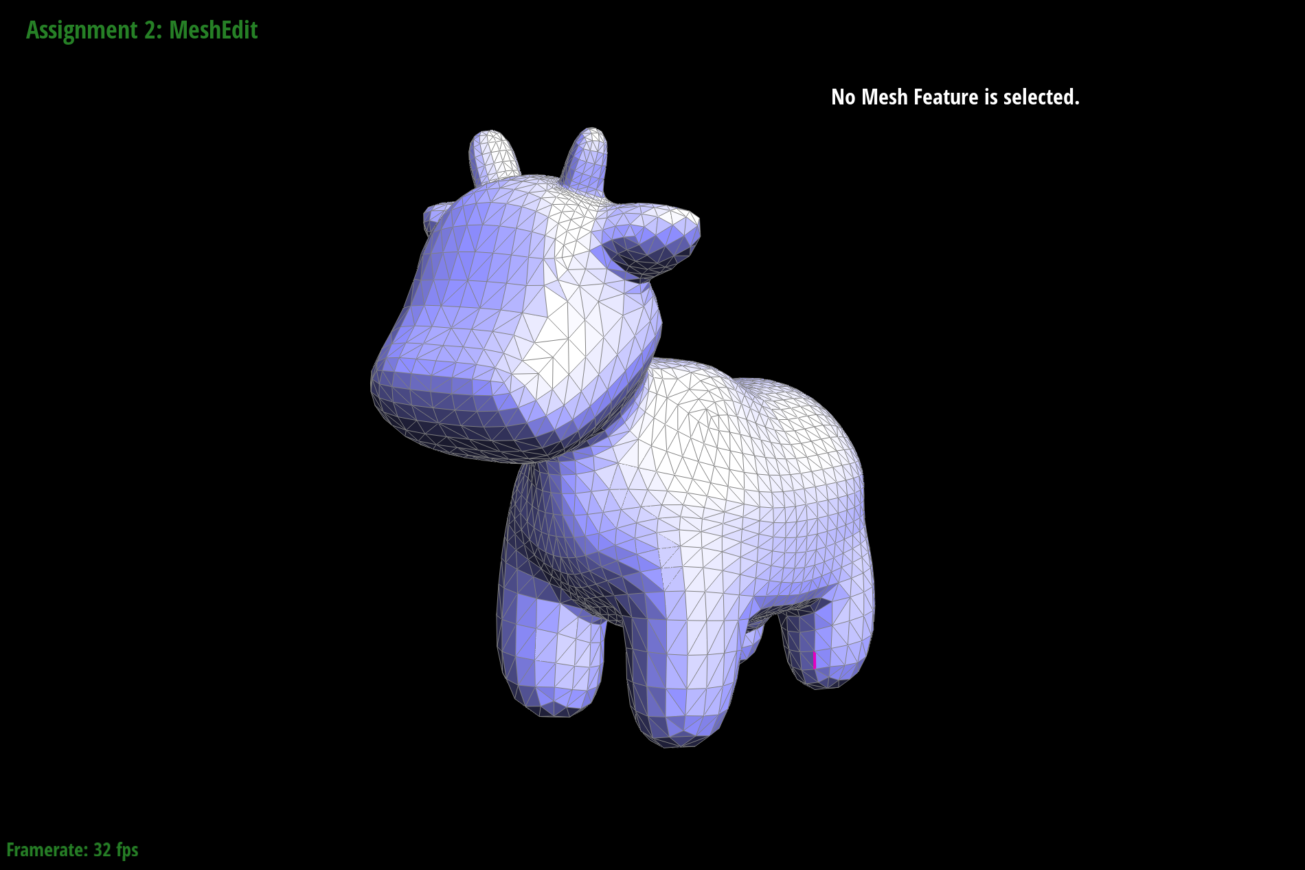
Cow Loop Subdivision 1
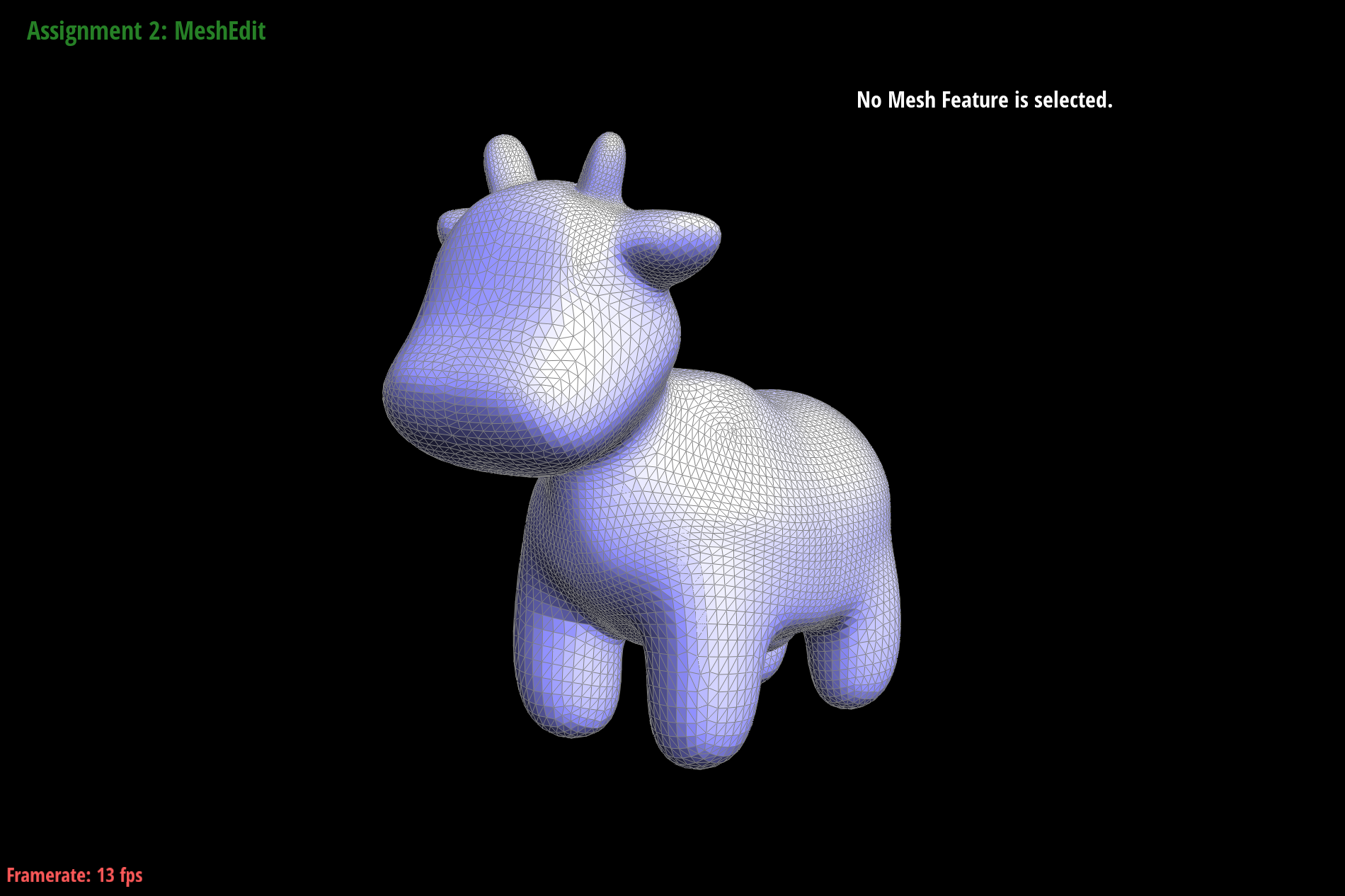
Cow Loop Subdivision 2
However with loop subdivision, this results in edges being lost as a result of increasing the number of triangles. There are some cases where this is ideal, but others where we'd want to keep the sharpness of corners and edges while still performing subdivision. In these cases, we could potentially pre-split some edges, specifically those that aren't edges and corners. We could potentially calculate whether something is an edge or corner by looking at the angle of two connecting faces, or have another flag that marks this information.
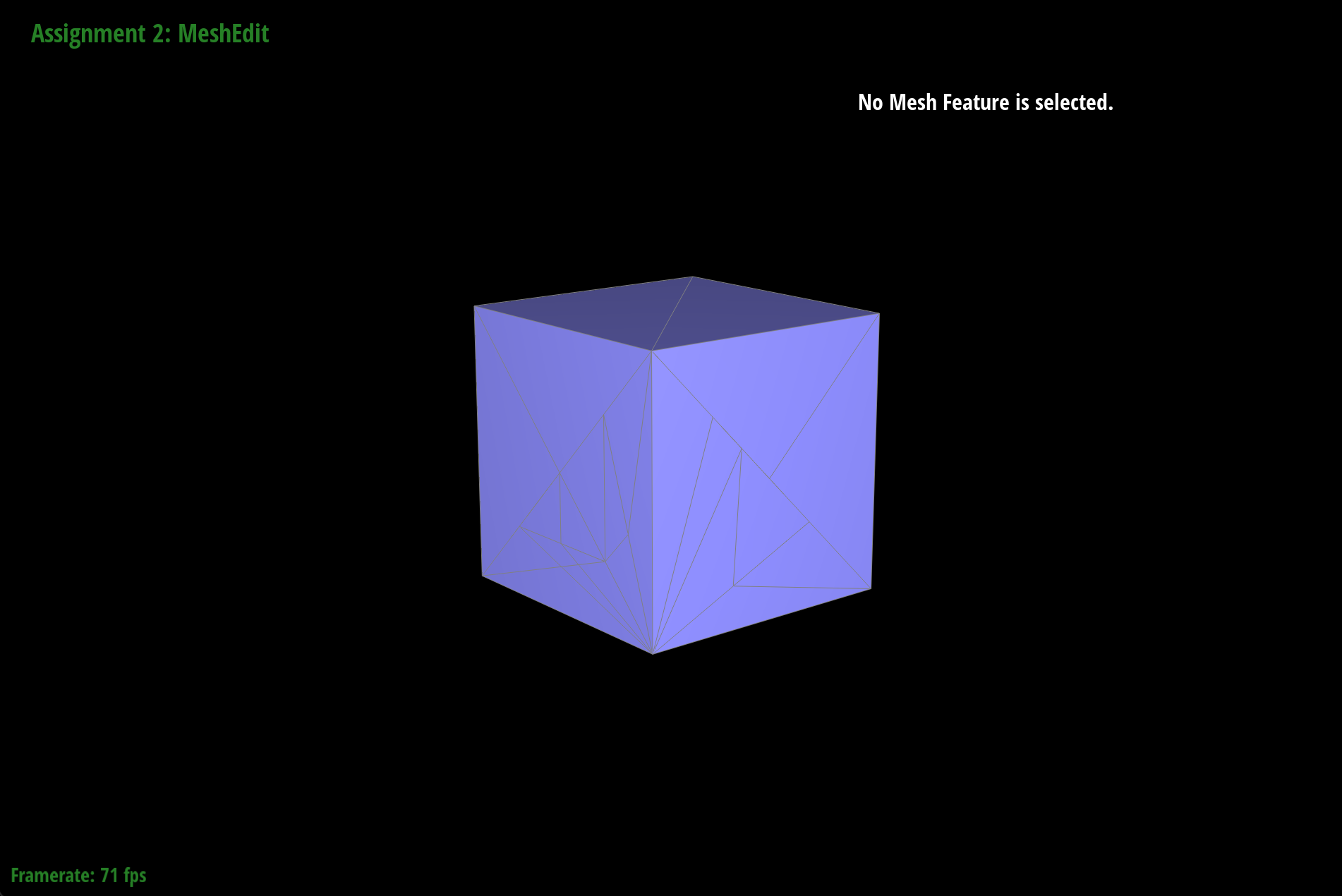
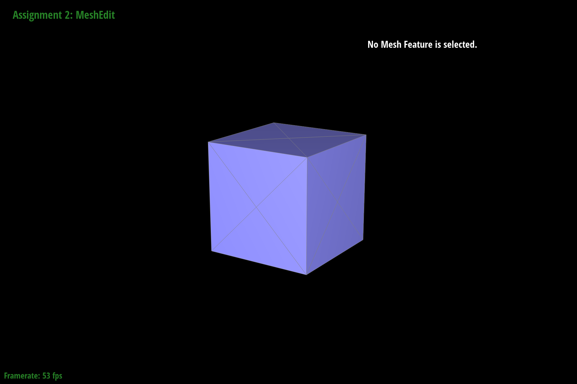
Here are screenshots of several iterations of loop subdivision on the cube.
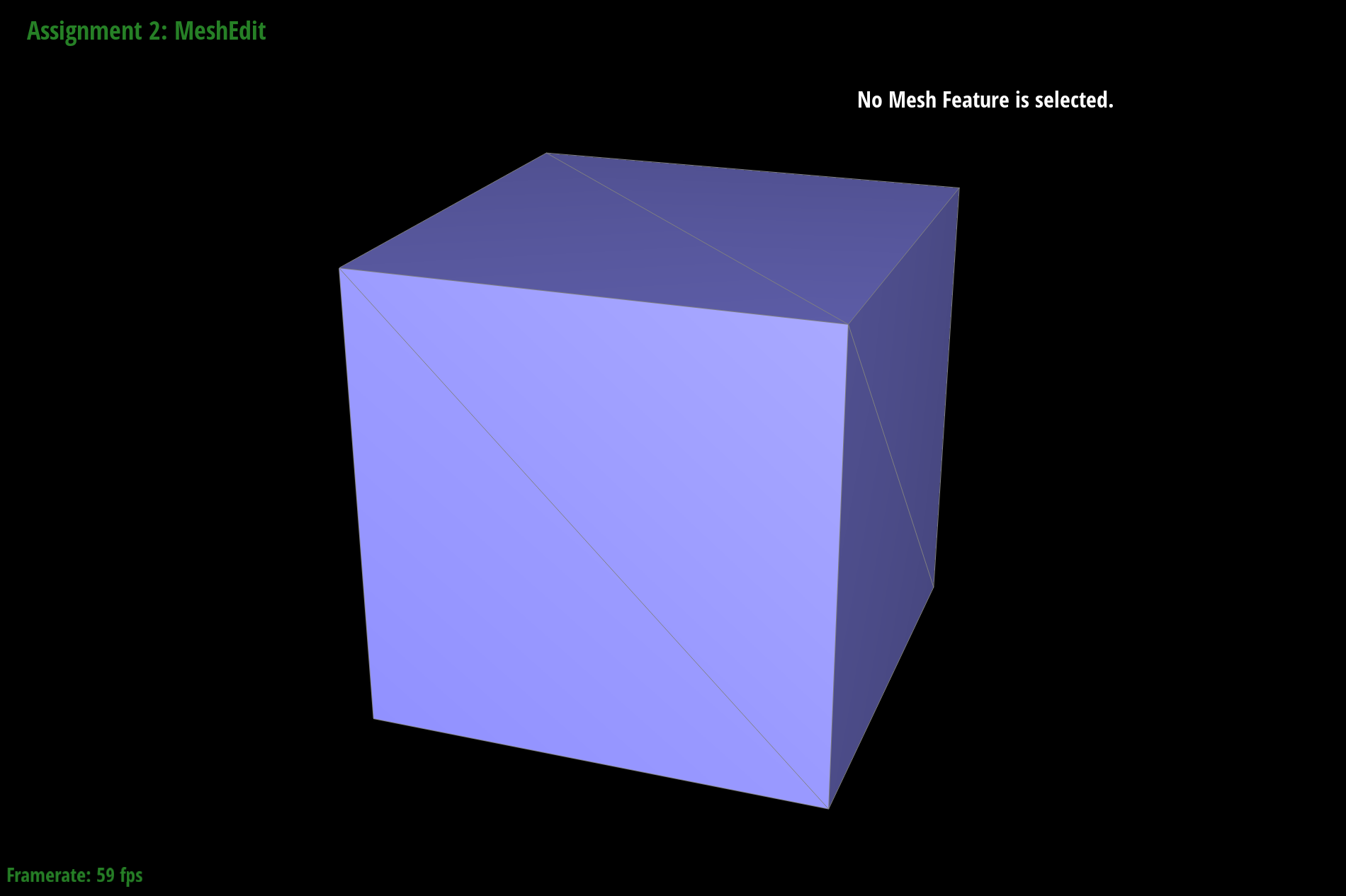
dae/teapot.dae loaded
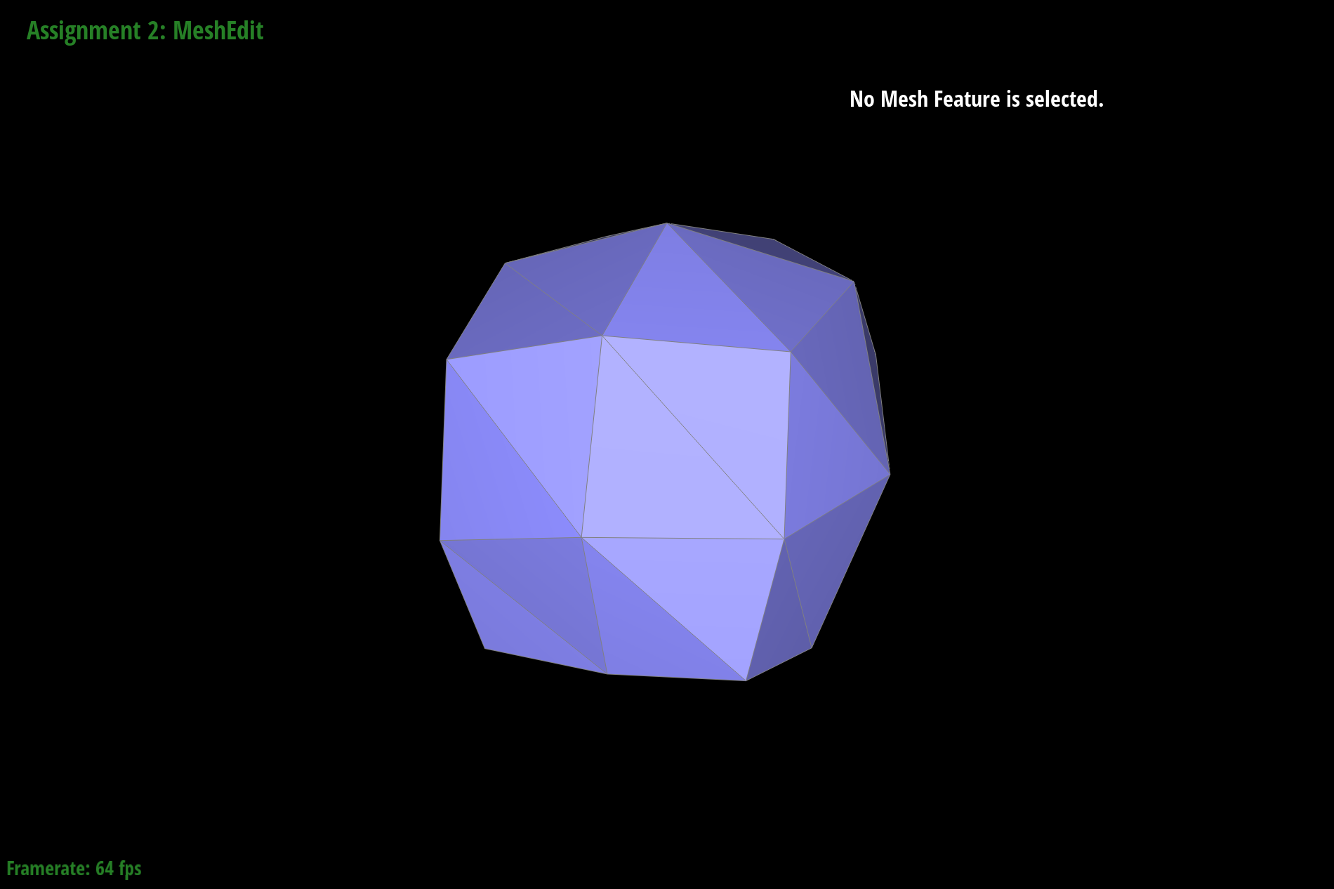
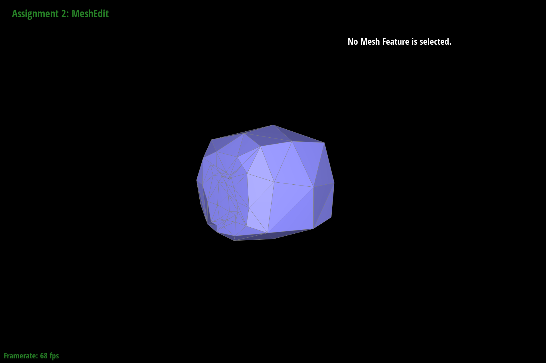
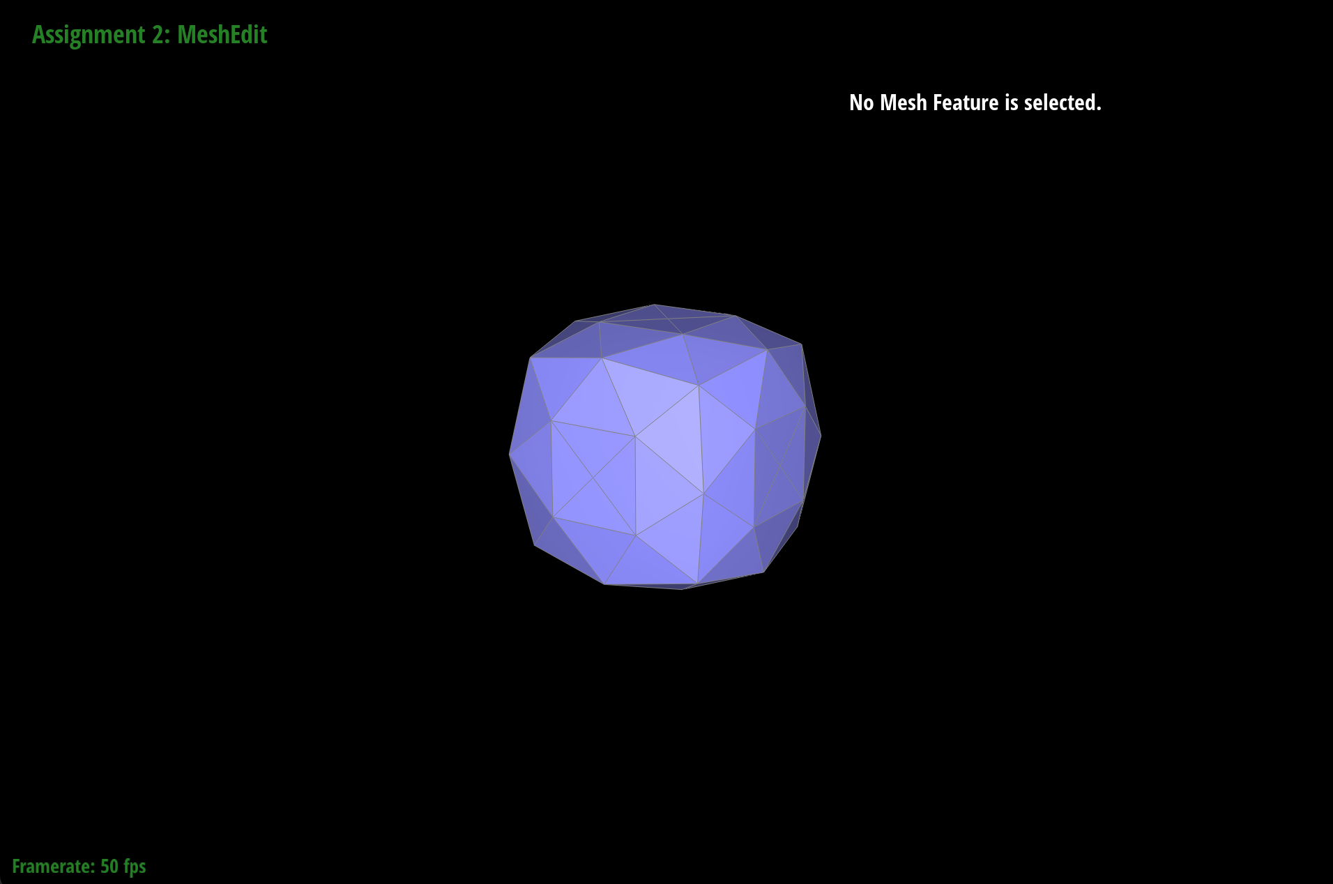
dae/teapot.dae loop subdivision step 1

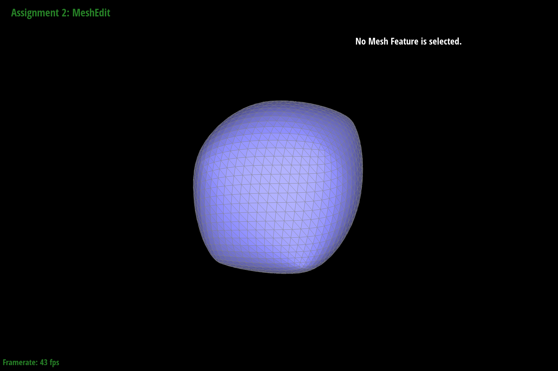
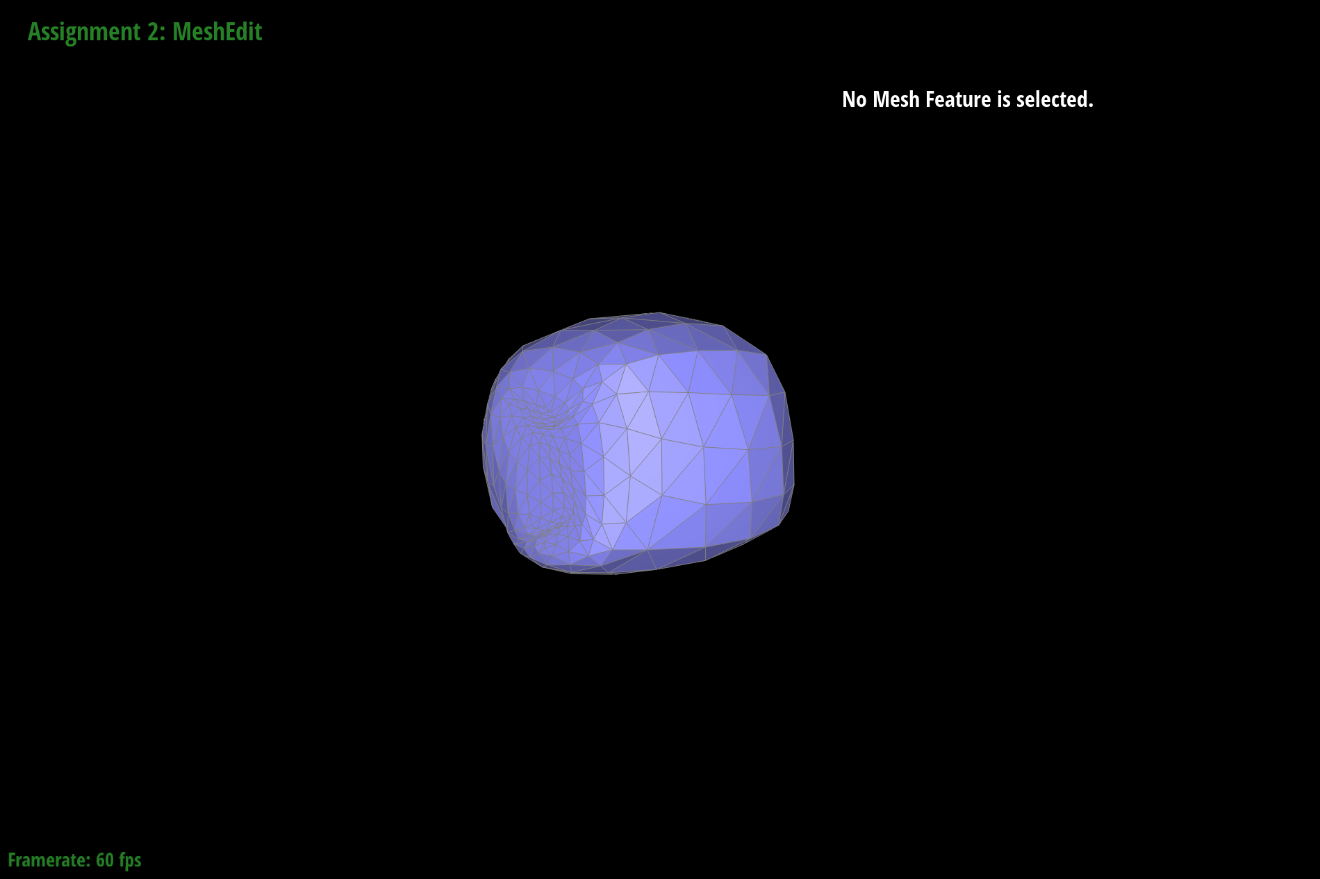
dae/teapot.dae loop subdivision step 2

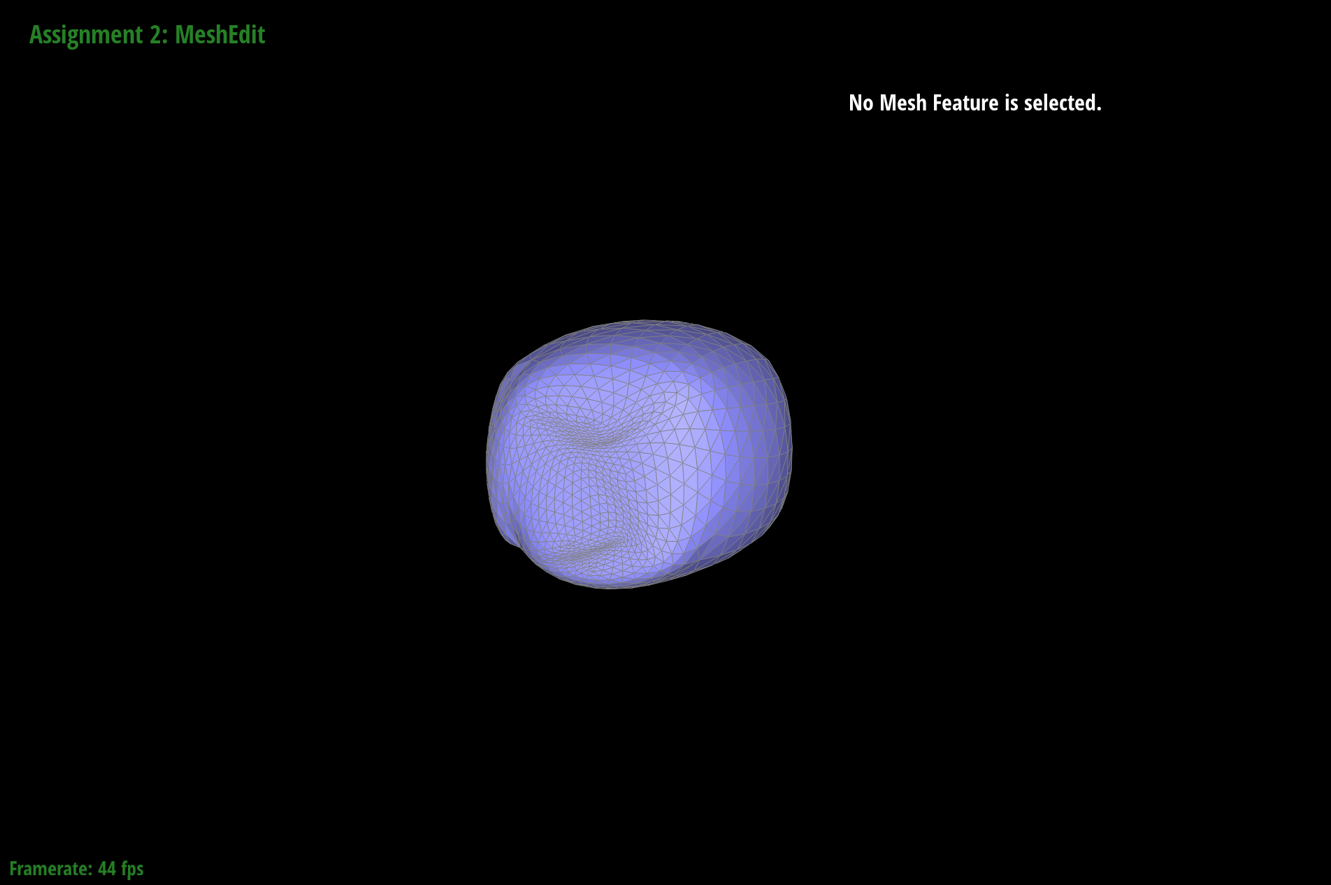
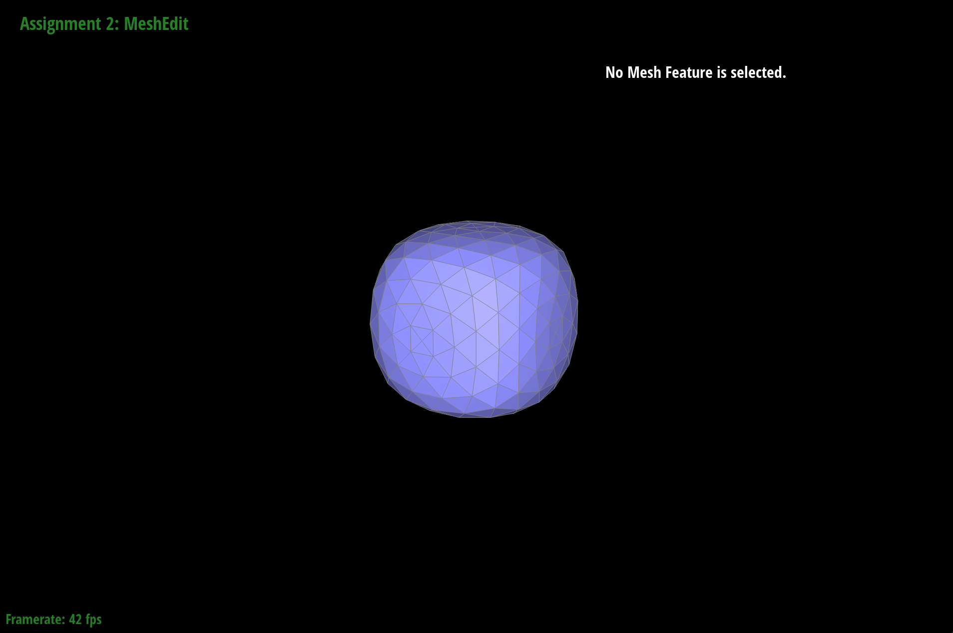
dae/teapot.dae loop subdivision step 3
dae/teapot.dae loop subdivision step 4
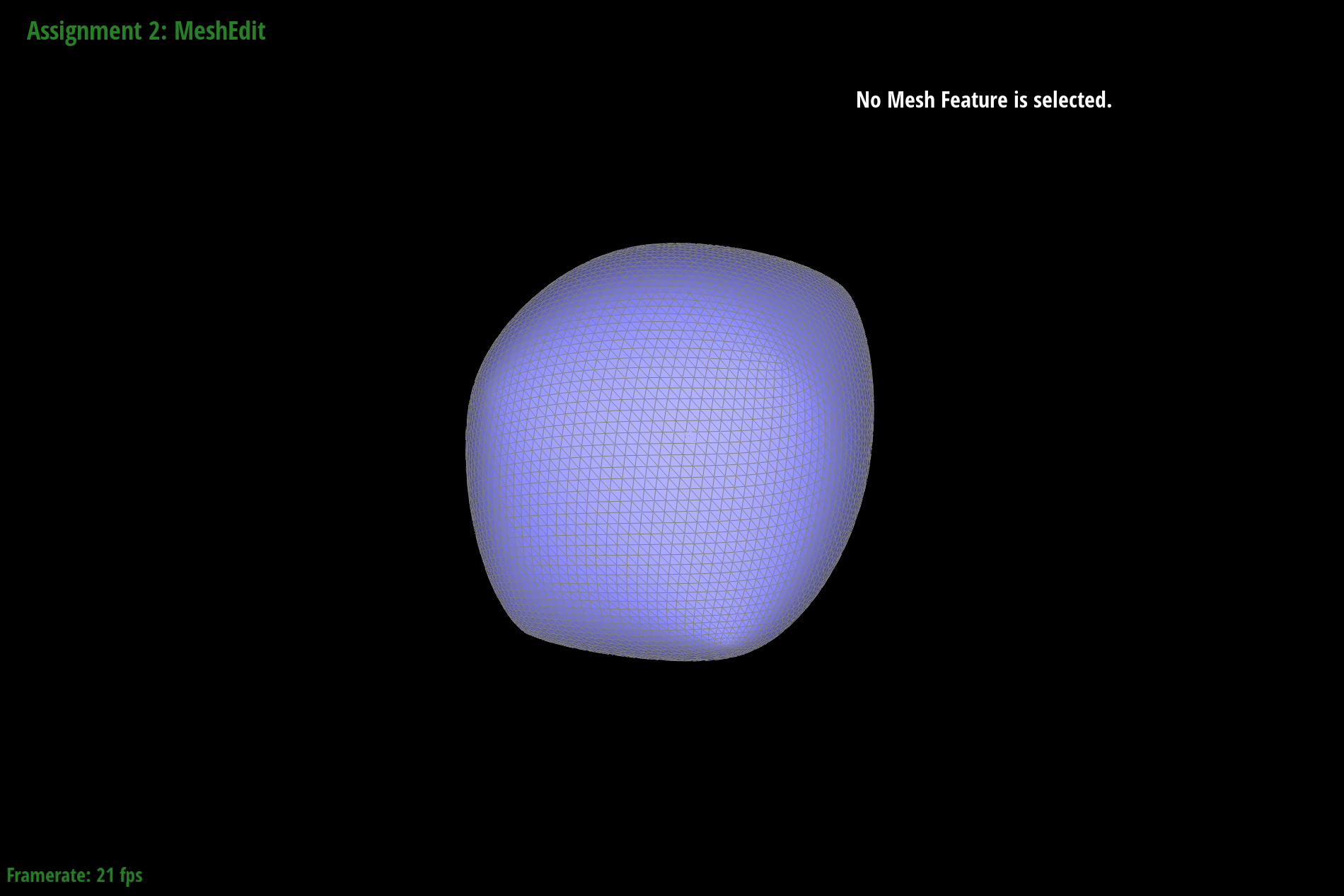
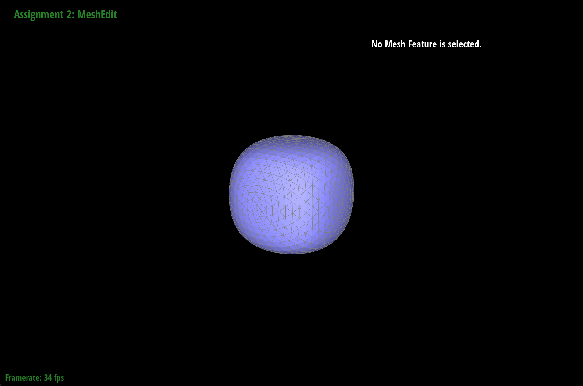
dae/teapot.dae loop subdivision step 5
As we can see, the cube becomes slightly asymmetric after repeated subdivisions. This could be because splitting and flipping the edges on the side of the cube have different results from splitting and flipping the edges that lay on the surface of the cube. For the cube specifically, it ends up being asymmetric because the faces of the cube only have one diagonal, instead of a symmetric two diagonals. This causes subdivisions to pull more in one direction than the other.
We attempted to reduce this by pre-splitting some edges. Below are some images of upsampling with pre-split edges which still shows that the sharpness remains despite the image smoothening out.
dae/teapot.dae with pre-split edges
dae/teapot.dae loop subdivision step 1
dae/teapot.dae loop subdivision step 2
dae/teapot.dae loop subdivision step 3
As a result, when we pre-process the splitting and flipping of edges, we can control which ones we do so that only the ones that keep the symmetry of the cube are edited. Here are screenshots of loop subdivision on the cube, but with edges pre-processed before the loop subdivision. In this case, we are splitting the edges on the faces of the cube before performing loop subdivision on the whole cube.
dae/teapot.dae pre-processed with one split on each face
dae/teapot.dae loop subdivision step 1 after pre-processing
dae/teapot.dae loop subdivision step 2 after pre-processing
dae/teapot.dae loop subdivision step 3 after pre-processing

dae/teapot.dae loop subdivision step 4 after pre-processing
dae/teapot.dae loop subdivision step 5 after pre-processing
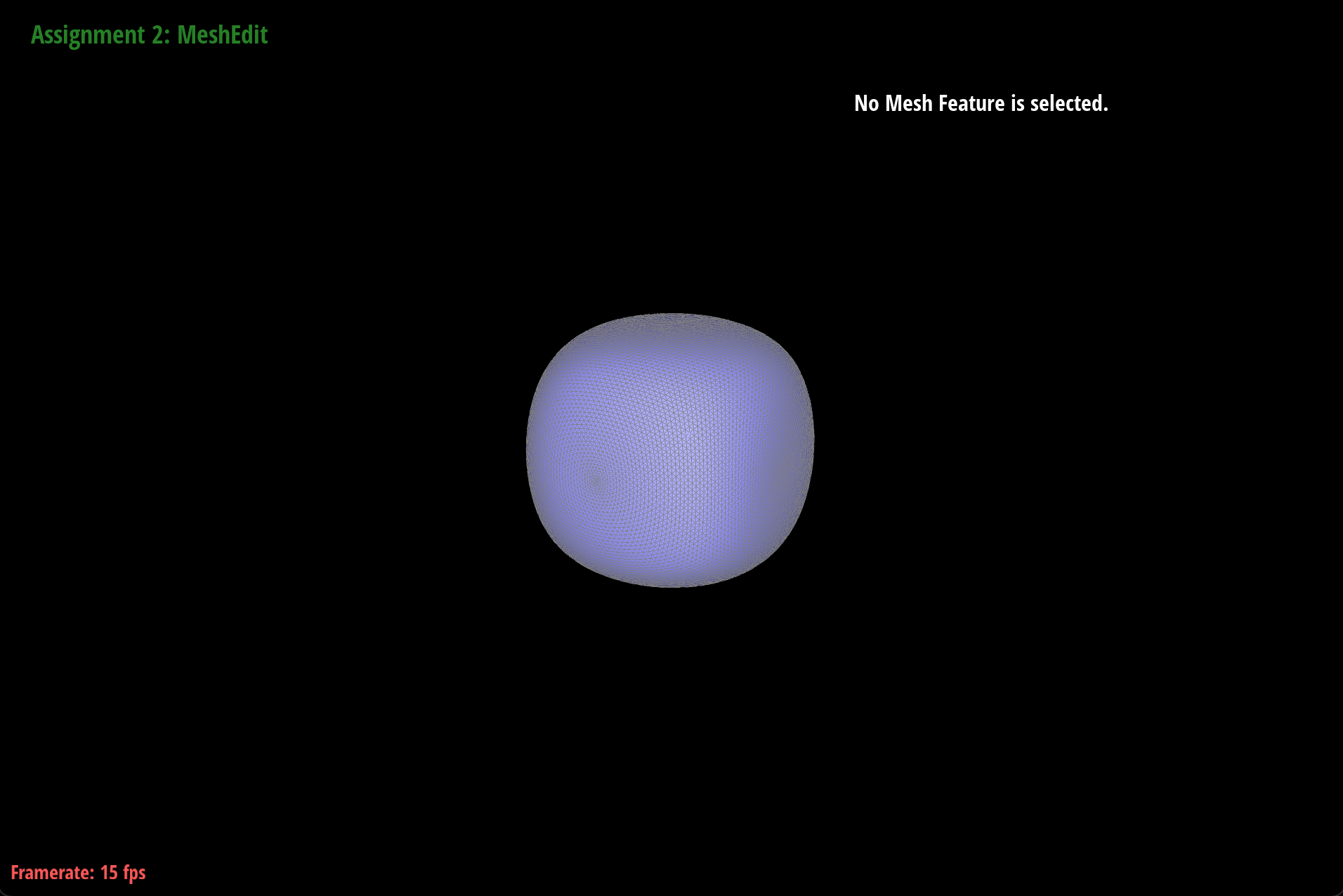
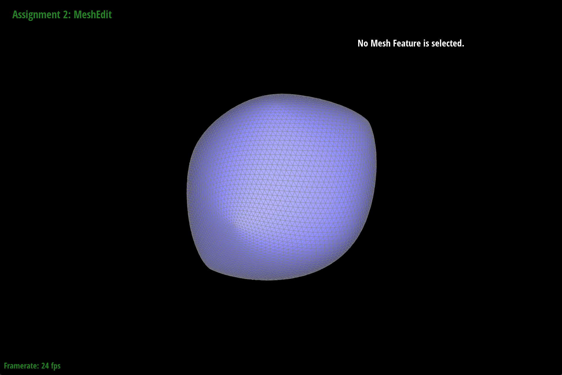
The difference in asymmetry is shown when comparing dae/teapot.dae images with no pre-processing and with pre-processing. The one on the left has weird bumps from the corners of the cube whereas the one on the right is more symmetrical and smooth.
dae/teapot.dae loop subdivision step 5, no pre-processing
dae/teapot.dae loop subdivision step 5, after pre-processing